An Introduction to Diffusion Models and Stable Diffusion

Introduction

Imagine a world where creativity transcends the limitations of brushes, clay, and canvas. It was in 2022, at Colorado’s State Fair art competition, that a groundbreaking entry defied the conventional boundaries of artistic creation. Jason M. Allen’s masterpiece, “Théâtre D’opéra Spatial” won the first prize and defied convention. Not through traditional means, but with the aid of an AI program called Midjourney, which uses a diffusion model to generate images. By turning a text prompt into a hyper-realistic image, Allen’s creation not only captivated the audience and judges but also set off a fierce backlash from artists who accused him of, essentially, cheating.

“Théâtre D’opéra Spatial” entry for the Colorado State Fair.

However, the rise of Midjourney and other AI advancements merely scratches the surface of what is possible with diffusion models. These generative models have become a force to be reckoned with, attracting attention and pushing the boundaries of image synthesis previously ruled by Generative Adversarial Networks (GANs) [1]. In fact, diffusion models are being said to be beating GANs on image synthesis [2].

In this article, we explore the theoretical foundations of diffusion models, uncovering their inner workings and understanding their fundamental components and remarkable effectiveness. Along the way, we’ll shine a spotlight on one of the most popular families of diffusion models: Stable Diffusion.

Join us as we uncover the secrets behind diffusion models’ success and how they are revolutionizing image generation. By the end, you’ll have a profound understanding of their transformative potential, inspiring the realm of AI-driven creativity.

Diffusion Models

Diffusion Models are generative models that learn from the data during training and generate similar examples based on what they have learned. These models draw inspiration from non-equilibrium thermodynamics and have achieved state-of-the-art quality in generating various forms of data. Some examples include generating high-quality images and even audio (e.g. Audio Diffusion Models [3]). If you are interested in how diffusion models can be applied in audio settings, check our blog on voice cloning. 

In a nutshell, Diffusion Models work by corrupting training data through the addition of Gaussian noise (called forward diffusion process), and then learning how to recover the original information by reversing this noising process step by step (called reverse diffusion process). Once trained, these models can generate new data by sampling random Gaussian noise and passing it through the learned denoising process.

Diffusion Models go beyond just creating high-quality images. They have gained popularity by addressing the well-known challenges associated with adversarial training in GANs. Diffusion Models offer advantages in terms of training stability, efficiency, scalability, and parallelization.

In the following sections, we’ll dive deeper into the fine details of Diffusion Models. We’ll explore the forward diffusion process, the reverse diffusion process, and an overview of the steps involved in the training process. Also, we’ll also gain an intuition on the calculation of the loss function. By examining these components, we’ll acquire a comprehensive understanding of how Diffusion Models function and how they achieve their impressive results.

Forward Diffusion Process

The forward diffusion process consists of gradually adding Gaussian noise to an input image step by step, for a total of T steps. At step 0 we have the original image, at step 1 a very slightly corrupted image which gets even more corrupted step by step until the whole information of the original image is lost.

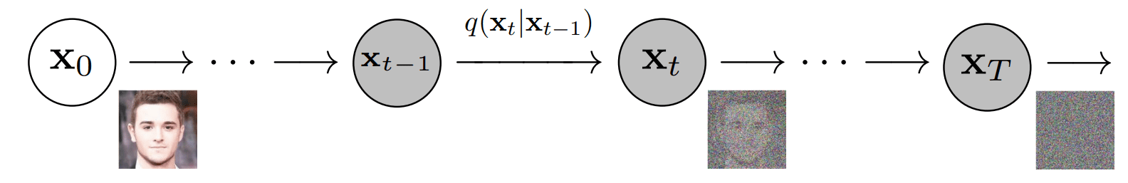
Forward diffusion process [4]

To formalize this process, we can view it as a fixed Markov chain with T steps, where the image at timestep t maps to its subsequent state at timestep t+1. As such, each step depends only on the previous one, allowing us to derive a closed-form formula to obtain the corrupted image at any desired timestep, bypassing the need for iterative computation.

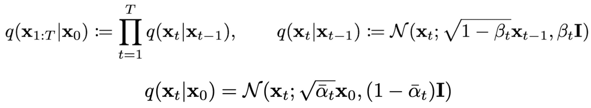
Forward diffusion formulation [4]

Consequently, this closed-form formula enables direct sampling of xₜ at any timestep, significantly accelerating the forward diffusion process.

Schedulers

In addition, the noise addition at each step follows a deliberate pattern. A Scheduler determines the amount of noise to be added. In the original Denoising Diffusion Probabilistic Models (DDPM) paper [4], the authors define a linear schedule ranging βₜ from 0.0001 at timestep 0 to 0.02 at timestep T. However, several alternatives gained popularity, such as the cosine schedule introduced in the Improved Denoising Diffusion Probabilistic Models paper [5].

For example, the following image shows the difference between using a linear schedule and cosine schedule for the forward diffusion process. A linear schedule is displayed in the first row, while the second row demonstrates the improved cosine schedule.

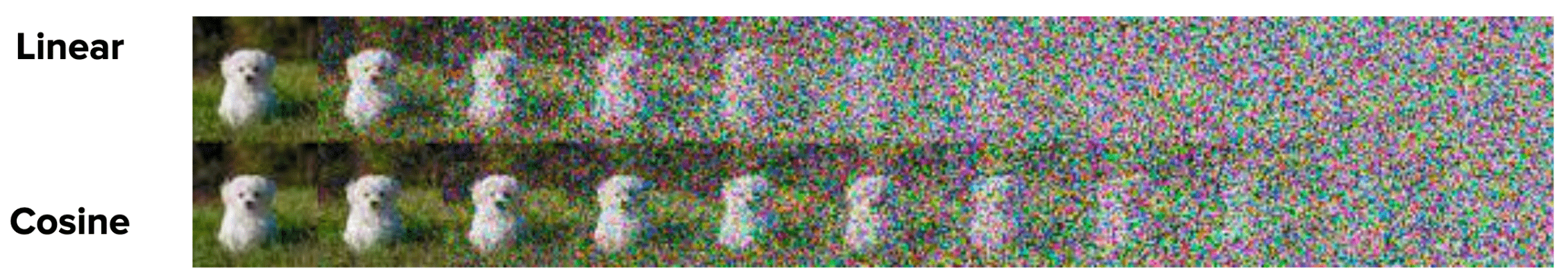
Linear and Cosine schedulers, extracted from the Improved DDPM paper [5]

The authors of the Improved DDPM paper argue that the cosine schedule offers superior performance. A linear schedule may lead to a rapid loss of information in the input image. As a result, this generally leads in an abrupt diffusion process. In contrast, the cosine schedule provides a smoother degradation. Hence, allowing the later steps to operate on images that are not completely overwhelmed by noise.

Reverse Diffusion Process

Conversely to the forward diffusion process, the reverse diffusion process poses a computational challenge as the formulation of q(xₜ₋₁|xₜ) becomes intractable or uncomputable. To address the challenges of the reverse diffusion process, deep learning models step into the spotlight, approximating this elusive reverse diffusion process with a neural network.

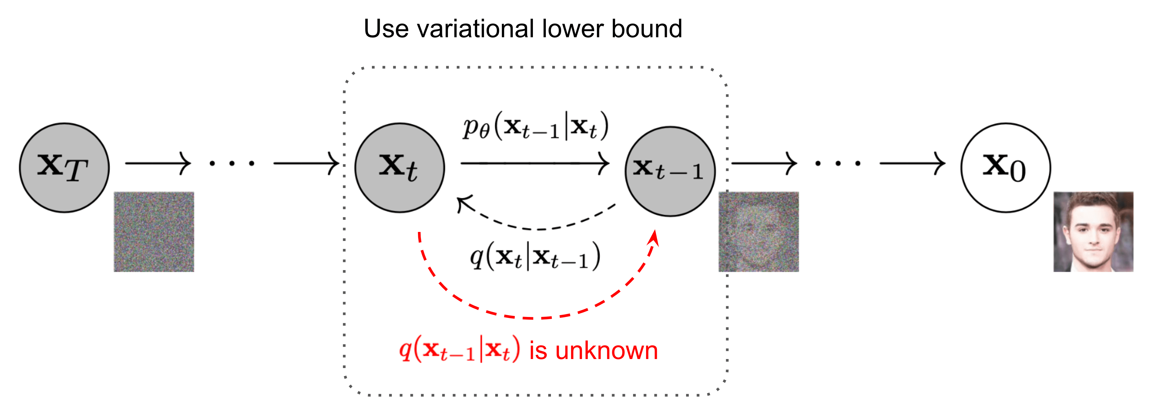
Reverse diffusion process [6]

Generally speaking, the role of this neural network is to predict the whole noise present in the image at a certain timestep t. Then, by comparing this prediction with the real noise added to the image, the network can be trained. At inference time, these networks still predict the whole noise present in the image at timestep t, and then just remove a fraction of the noise present according to the Scheduler used.

As a result, by predicting the noise at timestep t we may be tempted to try to retrieve the original image in just one step. However, some empirical experiments have shown that smaller steps are needed for achieving greater stability. Hence the need of removing just a fraction of the noise present at the image at timestep t in order to obtain the image at timestep t-1.

Some papers and blogs may be misleading in the sense that, from reading them, people tend to believe that the network predicts the noise added from timestep t-1 to timestep t. Although this can be clarified by looking at the code provided by their authors.

Neural Network Architecture

You may wonder about the architecture of this neural network. Generally speaking, Diffusion Models use some sort of U-Net variant to approximate the reverse diffusion process. This choice stems from the popularity of U-Net in the Computer Vision community. Also, seems a great fit considering that the only requirement is that the input and output of the Diffusion Model must maintain identical dimensionality, except from Super Resolution Diffusion Models [7].

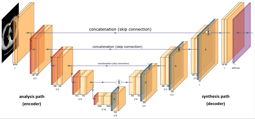
U-Net architecture [8]

Regarding the implementation details outlined in the DDPM paper, the main architectural choices involve:

• The encoder and decoder paths have the same number of levels, incorporating a bottleneck block between them.
• Each encoder stage consists of two Residual Blocks with convolutional downsampling, except for the final level.
• Each decoder stage consists of three Residual Blocks. Also, the authors define x2 nearest neighbor upsampling blocks with convolutions to restore the input from the previous level.
• The decoder path connects to each stage in the encoder path through skip connections.
• The use of attention modules at a single feature map resolution within the model.
• Additionally, the timestep t is encoded into a time embedding. This is quite similar to the Sinusoidal Positional Encoding presented in the Transformer paper [9].

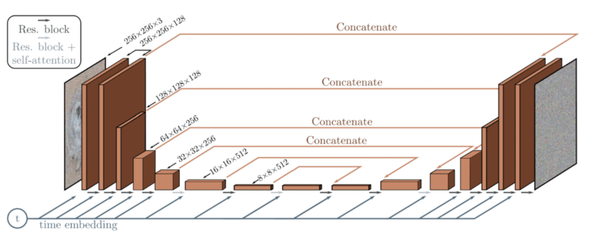
Diffusion Model architecture based on the U-Net [10]

These time embeddings help the neural network to gain certain information of at which state (step) is the image currently at. This is useful to know if more or less noise is currently present in the image, making the model subtract more or less noise. Generally speaking, in lower timsteps, the forward diffusion process adds less noise than in higher timesteps.

As an example, this is how the whole forward/reverse diffusion process looks like: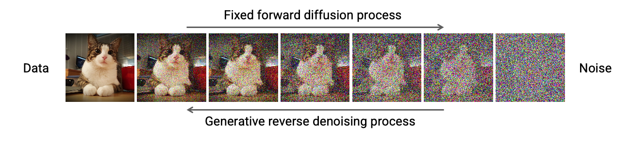

Forward and reverse diffusion process [11]

Loss Calculation

To train a Diffusion Model, the objective is to find the reverse Markov transitions that maximize the likelihood of the training data. This is equivalent to minimizing the Variational Lower Bound (VLB) on the negative log likelihood. Although it is called a lower bound, it is technically an upper bound, the negative of the Evidence Lower Bound (ELBO). However, we stick to the reference literature for consistency across different sources. In practice, maximizing the likelihood translates to minimizing the negative log likelihood

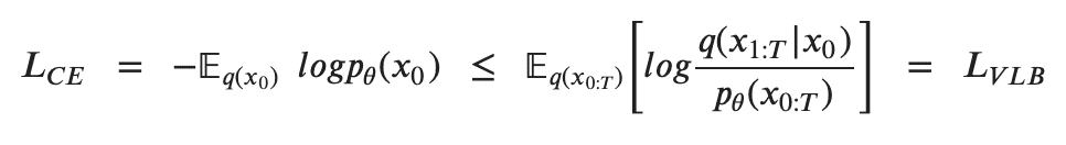
Jensen’s inequality for minimizing the cross entropy as the learning objective [6]

To convert each term in the equation to be analytically computable, the objective can be further rewritten to be a combination of several KL Divergence and entropy terms [12]. Additionally, For looking at a more detailed step by step formulation, visit Lilian Weng’s blog [6] on Diffusion Models.

Reformulation with KL Divergence

KL Divergence measures the asymmetrical statistical distance between probability distributions, quantifying how much one distribution P differs from a reference distribution Q. Formulating the VLB in terms of KL divergences is desirable since the transition distributions in the Markov chain are Gaussian, and the KL divergence between Gaussians has a closed form.

The mathematical representation of the KL divergence for continuous distributions is:

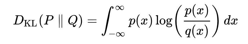
KL Divergence formulation [13]

But what does this look like in practice? We provide an example graph illustrating the KL divergence of a varying distribution P (blue distribution) from a reference distribution Q (red distribution). The green curve represents the function within the integral in the definition of the KL divergence, and the total area under the curve represents the value of the KL divergence of P from Q at a specific moment, displayed numerically.

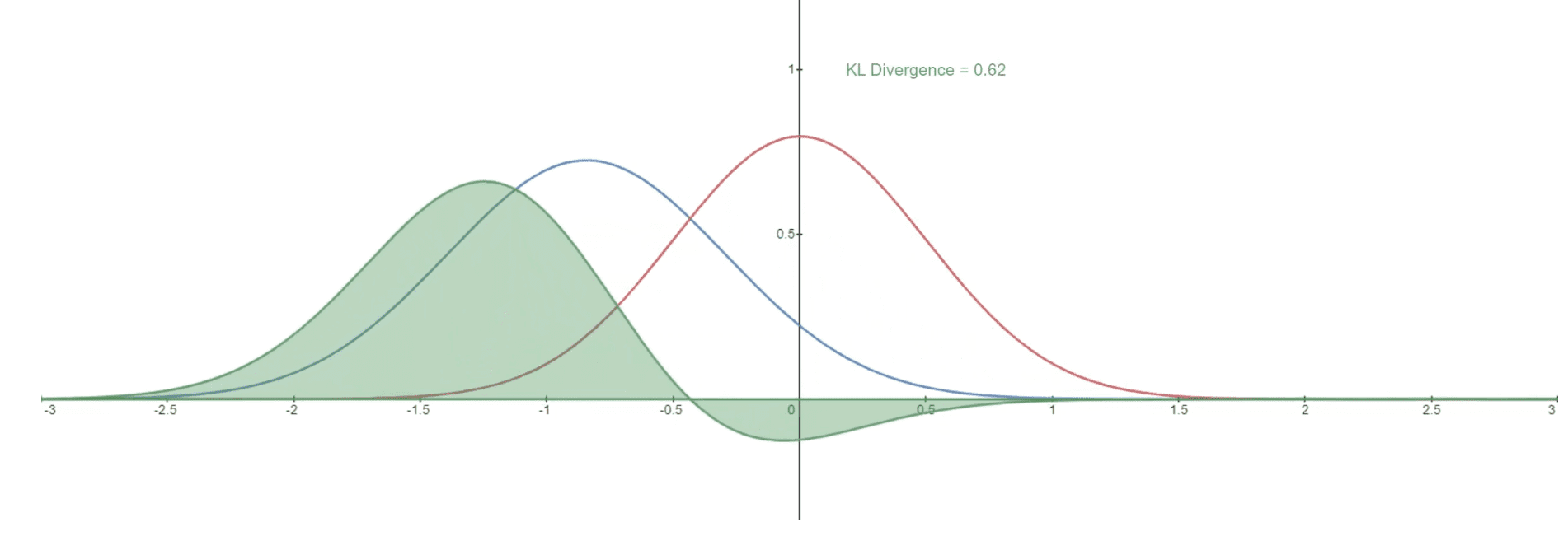
KL Divergence representation for two given distributions: Q (reference distribution) and P (varying distribution) [13]

The KL Divergence compares the Gaussian distributions in the diffusion training pipeline: the reference distribution from forward diffusion with added Gaussian noise, and the predicted noise during reverse diffusion.

We won’t dig deeply into Diffusion Models’ math. Nevertheless, we hope this helps as an overview of how these models calculate loss and update their parameters. The model predicts noise at a specific timestep t, using fixed standard deviation and real mean from forward diffusion, alongside mean and standard deviation of added noise. We calculate the KL divergence of images on these distributions. This computation spans all batch images, facilitating neural network backpropagation.

Training Process

In each batch of the training process, the following steps are taken:

1. Sampling a random timestep t for each training sample within the batch (e.g. images)
2. Adding Gaussian noise by using the closed-form formula, according to their timesteps t
3. Converting the timesteps into embeddings for feeding the U-Net or similar models (or other family of models)
4. Using the images with noise and time embeddings as input for predicting the noise present in the images
5. Comparing the predicted noise to the actual noise for calculating the loss function
6. Updating the Diffusion Model parameters via backpropagation using the loss function

This process repeats at each epoch, using the same images. However, different timesteps are usually sampled for each image at different epochs. This enables the model to learn reversing the diffusion process at any timestep, enhancing its adaptability

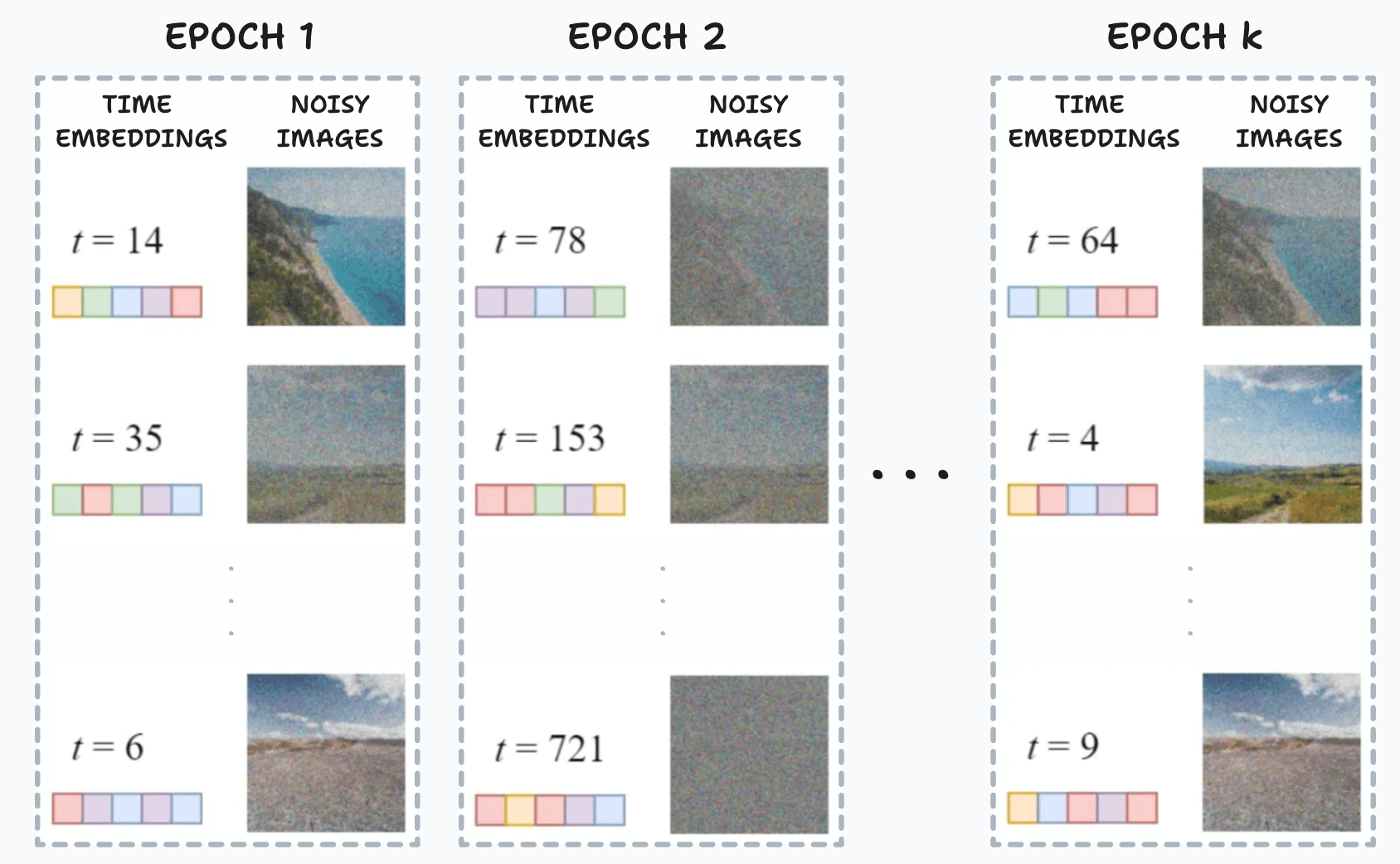
Representation of the corrupted images in a fixed batch during different epochs while training [14]

Sampling Process

For sampling new images, the difference lies in that we don’t have an input image. We sample random Gaussian noise and define how much steps of noise (T) to take for generating the new images. In each step, the Diffusion Model predict the whole noise present in the image, taking as input the current timestep. Then, it removes just a fraction of this predicted noise. We obtain our image generation result after T inference steps.

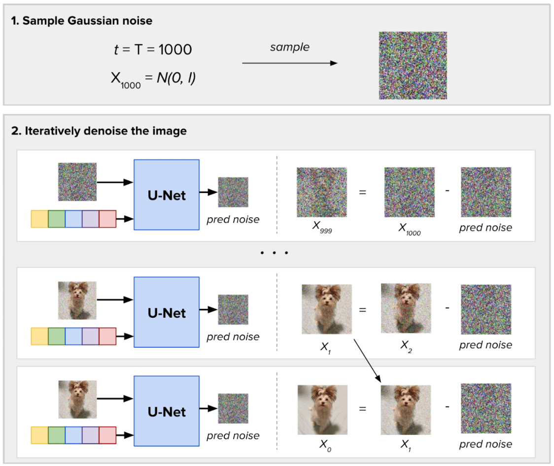
Denoising process for a single image

Stable Diffusion

The reverse diffusion process in traditional diffusion models involves iteratively passing a full-sized image through the U-Net architecture in order to obtain the final denoised result. However, this iterative nature presents challenges in terms of computational efficiency. This is emphasized when dealing with large image sizes and a high number of diffusion steps (T). The time required for denoising the image from Gaussian noise during sampling can become prohibitively long. To address this issue, a group of researchers proposed a novel approach called Stable Diffusion, originally known as Latent Diffusion Model (LDM) [15].

We’ll explore the main advances with regards to Diffusion Models presented in this paper: working with images in the latent space and conditioning.

Latent Diffusion Models

Stable Diffusion introduces a key modification by performing the diffusion process in the latent space. This works by using a trained Encoder E for encoding a full-size image to a lower dimension representation (latent space). Then making the forward diffusion process and the reverse diffusion process within the latent space. Later on, with a trained Decoder D, we can decode the image from its latent representation back to the pixel-space. For constructing the encoder and decoder, we can train some variant of a Variational AutoEncoder (VAE). This network is then decoupled for using both components separately.

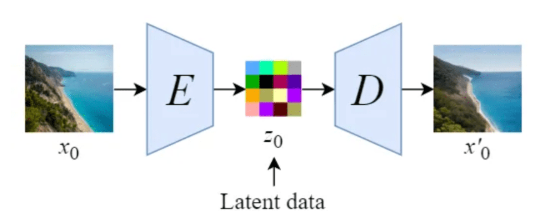
Illustration of an autoencoder as proposed by the Stable Diffusion paper [14]

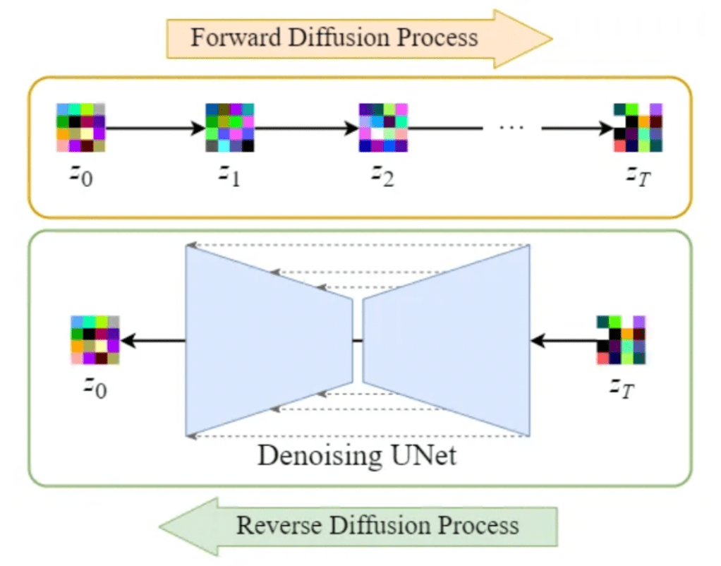
Illustration of an overview of the Stable Diffusion model within the latent space [14]

Shifting diffusion operations to the latent space in Stable Diffusion enhances speed and reduces costs. This advancement accelerates denoising and sampling processes, making it an efficient solution for high-quality image generation and stable training.

By leveraging the latent space, Stable Diffusion eases the computational burden in the reverse diffusion process. This enables quicker denoising of images, enhancing both speed and overall model stability and robustness.

Conditioning

Until then, generating images of a specific class was possible mainly through the addition of the class label in the input. Commonly known as Classifier Guidance. However, one of the standout features of the Stable Diffusion model, is its ability to generate images based on specific text prompts or other conditioning inputs. This is achieved by introducing conditioning mechanisms into the inner diffusion model, also seen in the literature as Classifier-Free Guidance (CFG) [16].

To enable conditioning, the denoising U-Net of the inner diffusion model makes use of a cross-attention mechanism. This allows the model to effectively incorporate conditioning information during the image generation (denoising) process.

The conditioning inputs can take various forms depending on the desired output:

• Text inputs are first transformed into embeddings through language models like BERT or CLIP. In the conditining, we map these embeddings into the U-Net using a Multi-Head Attention layer, represented as Q, K, and V in the diagram.
• Other conditioning inputs such as spatially aligned data such as semantic maps, images, or inpainting act similarly. However, the integration of these conditioning mechanismos is usually achieved through concatenation.

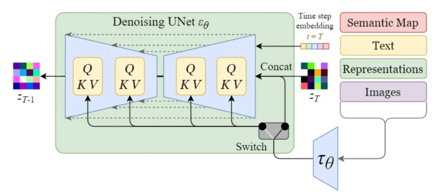
Conditioning mechanism within Stable Diffusion’s U-Net [14]

By incorporating conditioning mechanisms, the Stable Diffusion model expands its capabilities to generate images based on specific additional inputs. Text prompts, semantic maps, or additional images, enable more versatile and controlled image synthesis. By using prompt engineering, it’s possible to create even more compelling images. If you are interested in the best practices for applying prompt engineering for both Large Language Models and Stable Diffusion, check our blog on prompt engineering.

Architecture

In our journey through Latent Diffusion Models and the power of conditioning, we can notice a remarkable breakthrough in the world of image generation. Now, it’s time have a look at how the whole process of the Stable Diffusion looks like.

On the one hand, during training, the images (x₀) are encoded through the Encoder E, reaching the latent representation of the image (z₀). In the forward diffusion process, the image undergoes the addition of Gaussian noise, obtaining a noisy image (z_T). The image then passed through the U-Net, in order to predict the noise present in z_T. This comparison between the actual noise added in the forward diffusion and the prediction allows the calculation of the loss previously mentioned. With the calculated loss, we update the parameters of the U-Net through backpropagation.

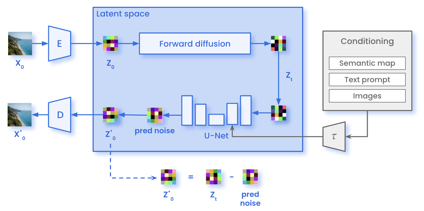
Stable Diffusion architecture while training

On the other hand, the forward diffusion process does not occur during sampling. We just sample Gaussian noise with the same dimensions present in the latent space (z_T). This noise passes through the U-Net for the specified number of inference steps T. At each step t, the U-Net predicts the whole noise present in the image. The model removes just a fraction of the predicted noise to obtain the representation of the image at timestep t-1. After all the T inference steps are iteratively, we obtain the representation within the latent space of the generated image (ẑ₀). Using the Decoder D, we can then transform that image from the latent space to the pixel-space (X̂₀).

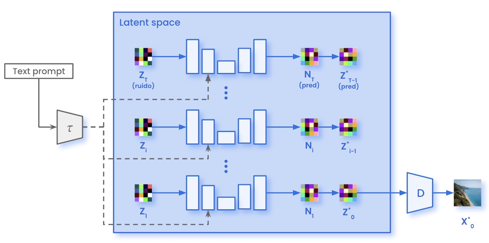
Stable Diffusion architecture while sampling

Use Cases

Diffusion Models offer versatile solutions to tackle various problems. Some of the most common use cases where Diffusion Models excel are:

• Image generation via prompting: generate images based on textual prompts or conditioning inputs, allowing for controlled and customizable image synthesis.
• Image super resolution: enhance the resolution and quality of low-resolution images, generating high-resolution versions with enhanced details and sharpness.
• Domain adaptation and style transfer: transfer the style or characteristics of one image or domain to another, enabling the adaptation of models trained on a source domain to perform well on a target domain with different visual characteristics.
• Image inpainting: fill in missing or corrupted parts of an image, reconstructing the missing details to create visually complete and coherent images.

• Image outpainting: expand the image outside its borders creating continuity and generating a bigger image.

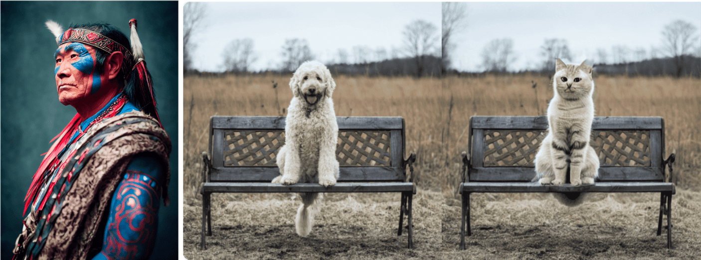
The first image is an example of what is possible to do with Midjourney, taken from the top section of their webpage. The second image shows an inpainting example for replacing the dog (via inpainting) with a cat (via prompting) [15].

Key Takeaways

In summary, here are the key takeaways we want you to have from reading this article:

• Diffusion Models consist of two processes: forward diffusion and reverse diffusion.
• The forward diffusion process consists of iteratively adding Gaussian noise. By using the closed-form formula in just one step, we remove the need of iterating. This enables faster generation of the corrupted images.
• The reverse diffusion process involves utilizing a neural network to approximate the denoising process. This process is iterative, step by step, until recovering the original image.
• Latent Diffusion Models (LDMs), improves the efficiency of diffusion-based image generation by performing the diffusion process in the latent space. This approach significantly speeds up the generation process, particularly for large images and longer diffusion steps.
• Some Diffusion Models offer the possibility of guiding the generation by using additional inputs. Texts and images are some of the common guiding inputs.
• Diffusion Models have found applications in various use cases. Some of these include: image generation via prompting, image inpainting, domain adaptation/style transfer, and image super resolution. These models offer versatile solutions for tasks ranging from creative image synthesis to image enhancement and restoration.

In conclusion, Diffusion Models became a new effective paradigm for image generation and manipulation. By combining the principles of diffusion processes with deep learning techniques, these models offer new avenues for generating high-quality images.

We hope that this blog serves for getting a deeper understanding on how Diffusion Models work. And stay stunned for more related content in future blogs!

References

• Generative Adversarial Networks Goodfellow et al. (2014)
• Denoising Diffusion Probabilistic Models (DDPM), Ho et al. (2020)
• Diffusion Models Beat GANs on Image Synthesis, Dhariwal and Nichol (2021)
• Improved Denoising Diffusion Probabilistic Models, Nichol and Dhariwal (2021)
• High-Resolution Image Synthesis with Latent Diffusion Models, Rombach et al. (2022)
• Classifier-Free Diffusion Guidance, Ho and Salimans (2022)
• Introduction to Diffusion Models for Machine Learning, AssemblyAI (2022)
• The Illustrated Stable Diffusion, Jay Alammar (2022)
• Diffusion Model Clearly Explained!, Steins (2022)
• Stable Diffusion Clearly Explained!, Steins (2023)
• An A.I.-Generated Picture Won an Art Prize. Artists Aren’t Happy, Kevin Roose (2022)
• How diffusion models work: the math from scratch, Karagiannakos and Adaloglouon (2022)
• What are Diffusion Models?, Lilian Weng (2022)