By Ignacio Mendizábal
Introduction
In the area of agricultural research, utilizing the power of satellite imagery has become a game-changer. These technologies provide valuable information that enables farmers, researchers, and industry professionals to make informed decisions, optimize resources, and maximize crop yields. However, working with satellite data has its own set of challenges and intricacies that we must carefully navigated.
Moreover, we’ve all witnessed how, on recent years, AI has taken over the world. We are without a doubt in a time of change. Everyday we see more & more applications of machine learning in all sorts of fields. So inevitably this brings up the question: what if we combined Machine Learning with satellite imagery?
In this blog, we explore the world of satellite imagery in agriculture and how to incorporate Machine Learning in the process. We’ll focus on the complexities of data preparation, models utilized, and potential applications. We’ll learn about the details of using satellite imagery to analyze crops, classify them, and estimate vegetation density to help farmers boost their productivity!
Use cases examples
The main question that might come to mind is: “How can we use satellite images in agriculture?” Well, there are many examples. Perhaps one of the most common use cases is identifying crop types across a region of interest. However, current research has opened a lot of new possibilities. We will now go over many examples, specially focusing on how these applications can boost productivity:
Crop classification & segmentation:
Imagine being able to identify, find & estimate the size of different crop types in a region of interest, using just a single satellite image of the desired region! One of the most common approaches for this consists on applying semantic segmentation models (such as Meta’s Segment Anything6) on each picture. This approach does a great job as our first shot, although we may need bigger & more complex models to achieve state-of-the-art accuracy. We can also use it to identify key geographical features such as water bodies or arid regions. This is by far the most common application.
Crop cycle tracking:
One key feature of satellite imagery is that it can provide insights about the vegetation of a specific region. This is possible thanks to specialized optical sensors that can capture information that cannot be seen with the naked eye. We will go into the details further in this blog. For now, keep in mind that, by using this information, it is possible to keep track of crop health to optimize farming practices.
Crop yield prediction:
What kind of information can we obtain if we study a region for a specific period of time? By analyzing multiple images taken over a wide timespan, it is possible to estimate crop yield for better decision making & planning for harvesting!
Analysis of crop phenological status:
Lastly, one of the most common practices in agriculture is phenotyping, which is usually time consuming and labor intensive. It is possible to monitor crop phenological states with satellite images by analyzing various characteristics such as flowering and maduration. It is possible to obtain information about these aspects from multispectral data. This grants the farmer a lot of information for better decision making.
Understanding Satellite data
We’ve now seen why satellite imagery can be useful in agriculture. Now, in order to see how it can help us, we must first understand the data it can provide us.
Multispectral imagery:
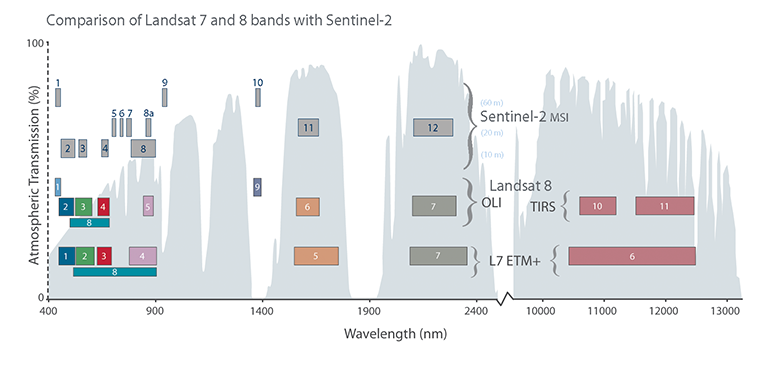
Currently, there are many types of satellites in orbit, each one with a wide range of sensors that provide different types of information. The most common type of data that satellites provide consists of color images of the earth’s surface, obtained by optical sensors that capture visible light. While this can certainly be useful, we can also obtain additional information if we analyze other parts of the electromagnetic spectrum, such as infrared. This is where the concept of “multispectral images” comes in.
Multispectral images are made by gathering light from different bands of frequencies. Unlike regular RGB images, which have just three color channels (red, green, and blue), multispectral images have lots of channels, each showing a different frequency band. We can see how different channels are distributed across different parts of the spectrum on figure 1.
Vegetation index (VI) & Land surface temperature (LST):
Many satellites are also able to measure the Land Surface Temperature (LST) of an area. That is, the temperature of the earth’s surface, ignoring atmospheric influence such as wind, humidity, etc. This can be very useful with various crops, and can also help us find optimal regions for agriculture.
But perhaps one of the most powerful tools that satellites can provide us is the ability to compute a vegetation index (VI). This index is obtained by analyzing red and infrared light components and can indicate the presence of vegetation in an area. There are many variations of this index, with NDVI being the most well known. Depending on our use case, we may opt for different implementations of this metric. But the key concept remains the same: measure the presence of vegetation in a region of interest.
Synthetic Aperture radars (SARs):
As you may have already noticed, satellites images are truly powerful. We saw how can we use it to measure temperature or vegetation density, which shows how much data we can obtain!
Unfortunately, all these data sources share the same limitation: they are obtained from optical sources. These sensors work by capturing light from the sun reflected off the earth’s surface. Because of this, there are many external factors that can affect the received data, such as weather and other unpredictable atmospheric conditions.
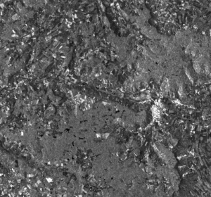
As an alternative, most satellites also count with Synthetic aperture radars or SARs. Radars work by transmitting radio waves towards an objective (in this case, the earth’s surface) and estimating how far it is based on how long it takes for the reflected pulse to come back. Radars can be used to map the earth’s surface by generating a “point-cloud” image. SARs are a special type of radar that takes advantage of the satellite’s movement as it orbits the earth to improve the image’s quality. Unlike visible light, radio waves can freely pass trough the earth atmosphere, which makes SAR images immune to weather conditions. Moreover, since no sunlight is needed, SARs can be used at any time, even at nighttime!
While all of this sounds like great news, it is important to note that, unlike traditional images, SAR data consists of just one channel, which is why most examples consists of grayscale images. This means we have less data to work with. An example of a SAR image is shown on figure 3:
Data sources
One of the most important aspects of any AI project is knowing where we can obtain data for our models. Nowadays, thanks to the effort of multiple agencies from all over the world, satellite imagery is more accessible than ever. We’ll now go over a few projects that provide easy access to different kinds of satellite data:
- The European Space Agency launched the “Sentinel-2” mission, which consists of 2 satellites that capture multispectral images of different parts of the globe. These images are publicly available through the Copernicus platform10 under a Creative Commons CC BY-SA 3.0 IGO license.
- The EarthExplorer9 platform was developed by the U.S. Geological Survey and provides images from a wide variety of missions, such as NASA’s Landsat. This information is free & consists mostly of RGB images, although other types of data can be found.
- The National Institute for Space Research of Brazil, in collaboration with China, has released a catalog of satellite images from South America & Africa11. Similar to previous cases, this information is available for free, under the Creative Commons Attribution-ShareAlike 4.0 International License.
As we can see, there are many options to choose from in order to extract data for our projects. All these efforts have also allowed many organizations to develop their own datasets. Some of which are also publicly available. Datasets such as EuroSat15, AgriFieldNet12 and the BigEarthNet13 benchmark provide labels for crop classification & segmentation, based on RGB & multispectral imagery.
We’ve now seen many ways satellite imagery can be used to improve agricultural productivity enhanced with machine learning. We’ve also seen what data satellites can provide us & how to access it. Now, we’ll use everything we’ve learned so far in a few experiments to show the power of these technologies!
Practical Examples
We’ve already discussed many applications for these technologies in agriculture. However, going through all of these cases would require more than a single blog post! We’ll now focus on two primary examples: crop classification and segmentation, since they are the most common.
Crop segmentation using a zero-shot segmentation model
We’ll now go through a simple example where we’ll use a segmentation network on a series of satellite images obtained from the Sentinel-2 mission in order to locate various plots & other key features across a specific region. We’ll use the Segment Anything6 model (SAM) as the segmentation network for these experiments. It is important to notice that we’re performing this test with a zero-shot model, meaning that our model hasn’t been trained with satellite images yet for this specific purpose yet.
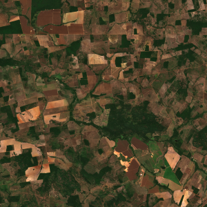
The images used in this demonstration were obtained from the Sentinel-2 mission, through the Copernicus platform. Since these are multispectral images composed of 12 channels, and SAM can only work with normal RGB images, we’ll have to choose 3 bands from the downloaded image to create an “RGB composite” that can be fed to the network. For our first experiment, we’ll choose the bands B-04, B-03 & B-02 as they correspond to red, green and blue light on the spectrum respectively. We can see an example of such image on figure 4:
We’ll now use SAM’s ViT-H model to obtain a segmentation mask on the given image. Keep in mind that, while this allows us to determine the location and size of crops & other key features, it does not identify each crop type. To achieve this, we’ll have to train our network to perform classification as well.
Once we process the image through the segmentation network, we obtain a mask like this:
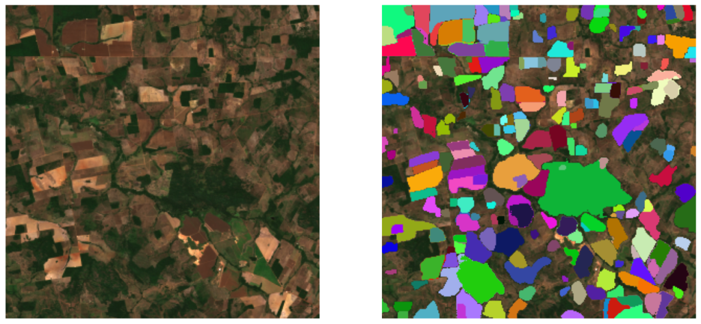
As we can see, the network is capable of identifying & segmenting different crops across the image, although it cannot distinguish each crop type for now. We could use this information to keep track of crop distribution across a specific region, which could be useful for analyzing available farmland. Remember this was done with a zero-shot model, imagine what we could achieve with further training!
Combining different spectral bands
Now, we’ve only used 3 of the 12 available spectral bands. What kind of information could we obtain from the rest of the channels? As we saw before, SAM can only process images with 3 channels, so a normal workaround is to create other combinations using different spectral bands. We can find many combinations on the Sentinel-hub repository16, suitable for various applications. These combinations are referred to as “RGB composites”.
For example, the “false color” composite, which consists of bands B08, B04 & B03 is commonly used to access plant density & health. Furthermore, a “short wave infrared” composite, which uses bands B12, B08 & B04 can give a great insight into how much water is present in plants and soil, which can be useful for detecting fire damage. We can experiment with these composites by combining other bands & feeding the resulting image through the segmentation network to see what results we get. For this proof of concept, we mainly used 3 RGB composites. Each of these, as well as the obtained results, are shown below:
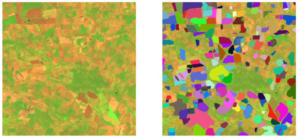
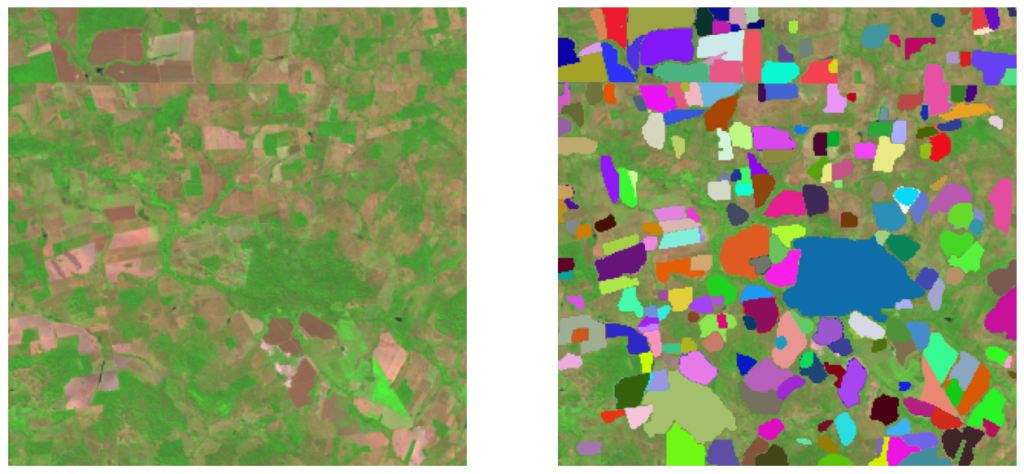
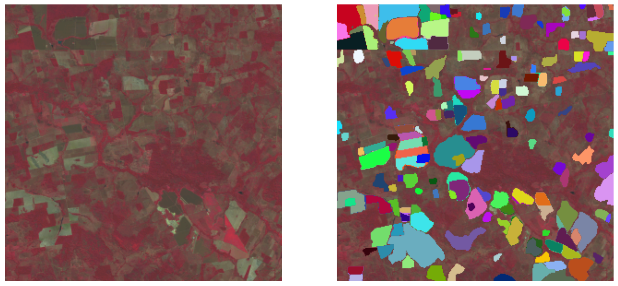
We can see that the obtained masks differ depending on the RGB composite used. This shows how each of these bands hold different information that can be interpreted differently by our model. For some applications, using one of these composites might be enough. However, there’s still a lot of information we can make use of.
Our next steps would be to experiment with these spectral bands, trying different combinations and adding different processing techniques to see if we can improve the results. We can also try with different segmentation models, or even training our own custom model. As we can see, there are many possibilities, the world of satellite imagery is truly powerful!
Crop classification with Time series of satellite images
As we’ve seen before, crop classification is one of the most common use cases. However, unlike our previous example, it is usually a much more complicated task. This is because to the light reflected from crops usually varies over time, which makes classification way harder with just a single image.
As an alternative, many state-of-the-art proposals usually involve the use of time series of satellite images. By having multiple pictures of the same crop across a specific time period, we can see how light reflectance evolves. We can use this information to determine the crop type, as different crops usually have different light reflectances.
To demonstrate this, we can see an example of the variation of the light reflectance of winter rapeseed crops over time across different spectral bands on the following graph:
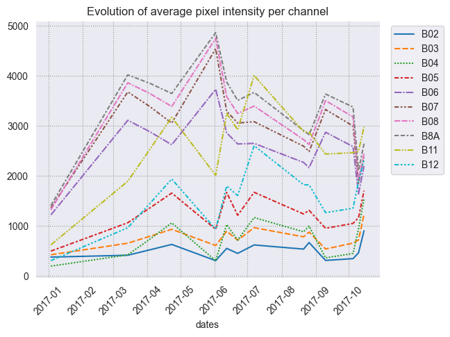
Source: Garnot, Vivien Sainte Fare, et al. 1
This clearly shows that, in order to correctly classify crops, we must make use of time-series of data. As such, many machine learning models for this task usually implement architectures for sequential data, such as transformers. This makes these models more computationally expensive than traditional fully connected or convolutional neural networks, but provide considerably better results.
Current benchmarks
Thanks to the effort of many organizations that have worked on multiple crop classification benchmarks, there is a wide variety of models to choose from. One example is this implementation by Garnot et al1 which claims to achieve up to 94.2% overall accuracy on classification tasks. While this is certainly impressive, one downside is the amount of time it takes to generate the necessary training data. Thankfully, the authors released a set of pre-trained weights ready for inference, as well as the original training dataset. With these resources, we can set up our own crop classification pipeline in no time!
We’ve performed our custom tests with this model, using a small dataset of 500 crops. The results were quite promising. Not only we obtained an accuracy of 94%, but also overall good values of precision & recall for most classes: for example, the precision score for sunflower and spring durum wheat crops was 85,7% and 98,3% respectively. On the other hand, other crop types such as cereal had lower precision scores of up to 55%. This is most likely due to data imbalance in our dataset.
Other promising works include this implementation of Vision Transformers for crop classification via time series of satellite images, by Michail Tarasiou et al2. This model can also be used for crop segmentation, which is a great plus. However, its accuracy is slightly slower than our previous model, with a score of 87,1%.
As we can see, crop classification is indeed a complex task. But it is an incredibly powerful tool. Especially when combined with our previous segmentation experiments.
Final Thoughts
In this blog, we got a first glance into the world of satellite imagery and its applications on agriculture. We’ve looked into the data it offers and figured out how to get our hands on it. We saw its true potential when combined with machine learning. And most importantly, we saw the wide array of possibilities that these two tools can offer when combined & used together.
It is clear that satellite imagery has a lot of challenges to overcome. But thanks to the constant improvement of machine learning models, we can expect to obtain better results in the future!
References:
- V. S. F. Garnot, L. Landrieu, S. Giordano, N. Chehata, Satellite image time series classification with pixel-set encoders and temporal self-attention, arXiv:1911.07757, 2020.
- M. Tarasiou, E. Chavez, S. Zafeiriou, ViTs for SITS: Vision Transformers for Satellite Image Time Series, arXiv:2301.04944, 2023.
- Quantum, Crop type classification with satellite imagery, Medium.com, August 14, 2022.
- A. H. Khan, M. M. Fraz, M. Shahzad, Deep Learning Based Land Cover and Crop Type Classification: A Comparative Study, 2021.
- R. C. Daudt, B. L. Saux, A. Boulch, Y. Gousseau, Urban change detection for multispectral earth observation using convolutional neural networks, arXiv:1810.08468, 2018.
- Alexander Kirillov et al., Segment Anything, Meta AI Research, arXiv:2304.02643, 2023.
- User Guides – Sentinel-2 MSI – Overview – Sentinel Online, Sentinel Online, Accessed 10 Oct. 2023.
- Comparison of Sentinel-2 and Landsat Active, USGS EROS Archive, U.S. Geological Survey, 1 Mar. 2019.
- EarthExplorer, U.S. Geological Survey, Accessed 10 Oct. 2023.
- Copernicus Browser, European Space Agency, Accessed 5 Feb. 2024
- Catálogo de Imagens, INPE, Accessed 10 Oct. 2023.
- AgriFieldNet India Challenge, Zindi, Accessed 10 Oct. 2023.
- G. Sumbul, M. Charfuelan, B. Demir, V. Markl, BigEarthNet: A Large-Scale Benchmark Archive for Remote Sensing Image Understanding, arXiv:1902.06148, 2019.
- Simple RGB Composites (Sentinel-2), Sentinel-Hub. Accessed 10 Oct. 2023.
- What Is Synthetic Aperture Radar?, Earth Science Data Systems, NASA, 10 Apr. 2020.
- What Is NDVI (Normalized Difference Vegetation Index)?, GISGeography, 14 July 2023.
- Land Surface Temperature, Copernicus Global Land Service, 30 Mar. 2023.

