By Agustina Gomez
Introduction
Are you a business owner or an IT professional? If so, you’re likely always on the hunt for ways to enhance your product, service, or algorithm. Changes can be risky, especially in productive environments. It’s hard to predict whether they will benefit your business. This is where A/B testing becomes valuable.
A/B testing is a powerful tool. It lets you test different versions of your product, service, or algorithm. This helps to identify whether a change will have a positive impact. A/B testing uses probability theory to support data-driven decision making. This can lead to better engagement, higher conversion rates, and increased revenue.
In this blog, we will explore the basics of A/B testing, covering important concepts and statistical methods. We will begin by discussing the importance of selecting the appropriate sample size. We will use the statsmodel library to calculate the sample size for proportions and means. Then we will delve into performing a z-test for proportions and means, and explore how to use bootstrapping for A/B testing. Finally, we will analyze some possible outcomes of A/B testing and how to interpret the results.
Latency test at Google
In 2009, Google ran an A/B test to study how website latency affects user behavior. For this test, Google divided their user traffic randomly into two groups. One group viewed pages that loaded at normal speed. The other group viewed pages that had a deliberate delay of 100-400 milliseconds.
The test results were surprising. Even a small delay of just 100 milliseconds led to a measurable decrease in user engagement. The group that experienced the delayed pages performed 0.2% to 0.6% worse on various user engagement metrics. These included search queries and ad clicks.
These findings made Google realize that website latency significantly affects user engagement. Even minor improvements in page speed can enhance user behavior considerably. The tech industry now widely accepts this insight. Many companies now invest heavily in optimizing the performance of their websites and applications. This improves user engagement and retention.
A Practical Example of the Process
Let’s consider a practical example. Suppose you have a digital product, like a website. You want to test whether a new design for your landing page will improve conversions or click-through rates. The variables you consider will depend on your specific business application. Two commonly identified types are binary or continuous.
Binary variables can represent whether a user has installed an application or not. These are used to calculate conversion rates (proportions). Continuous variables can be associated with an average, such as a cost per click.
In this example, we’ll test whether the new landing page improves click-through rates (CTR). However, we’ll consider both cases for the rest of the blog.
Running an A/B Test
To run an A/B test, you first need to define two groups: treatment and control. You then assign individuals to each group randomly. The size of each group is not trivial and we’ll discuss this later. The treatment group gets the variant to be tested, while the other group remains the same. While the experiment is running, it’s crucial to monitor not just the primary metric you want to optimize, such as CTR. You should also keep an eye on other relevant metrics that should stay consistent. This ensures that any changes made to improve the primary metric do not negatively impact other key metrics.
After you’ve collected your samples, you need to analyze your A/B test’s results. Looking at the results, we see that the treatment group had a 1% higher score than the control group. This might seem like a positive result initially. However, it’s crucial to ensure that this result is statistically significant. Statistical significance helps quantify whether a result is likely due to chance or a factor of interest. When analyzing the results of an experiment from a sample, it’s possible for one group to appear to outperform the other due to chance. But this may not be the case. To avoid drawing false conclusions by comparing two absolute values, we perform a hypothesis test. This lets us conclude with some confidence that the results obtained are not due to chance alone.
Why Hypothesis testing
“Hypothesis testing provides an objective framework for making decisions using probabilistic methods, rather than relying on subjective impressions. People can form different opinions by looking at data, but a hypothesis test provides a uniform decision-making criterion that is consistent for all people.” – Rosner, B. Fundamentals of Biostatistics.
In A/B testing, we will test whether there is a significant change in our metric after implementing the variant and also the magnitude of the effect. Typically, we will formulate hypotheses of the following types:
- Null hypothesis (H0): The metric is the same for both groups. I.e. mean_treatment = mean_control.
- Alternative hypothesis (H1): The metric is different. I.e. mean_treatment != mean_control
The process
The standard procedure for hypothesis testing is to define the null and alternative hypotheses. We then determine whether we support or reject the null hypothesis. To do this, we compute a test statistic. This measures how far the sample estimate is from the hypothesized value under the null hypothesis. In this context, it measures how far the computed difference between the two groups is from zero. This is because the null hypothesis is that the metric is the same for the two groups.
We then use the test statistic to calculate the p-value. This represents the probability of observing the result if the null hypothesis is true. In other words, it represents the probability of obtaining a difference such as the one observed. This assumes that the metric is the same for both groups. If the p-value is less than a certain level of significance (also known as alpha), then we reject the null hypothesis in favor of the alternative hypothesis. The lower the p-value, the less likely it is that the results are due to chance alone. However, if the p-value is greater than or equal to the significance level, we do not reject the null hypothesis. This indicates that there is not enough evidence to conclude that the groups or variables are different.
Possible results
All results in a hypothesis-testing situation generally refer to the null hypothesis. Thus, if we decide that H0 is true, we say that we accept H0. If we decide that H1 is true, then we say that H0 is not true, or equivalently, that we reject H0. So there are four possible outcomes:
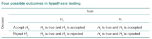
– Rosner, B. Fundamentals of Biostatistics (7th ed.), p. 204
Ideally, we want to accept H0 whenever it is truly true and reject it otherwise. In this context of decision making under uncertainty, we can make two types of errors. This is because we are working with a sample and want to test whether these results can be extrapolated to the population.
Types of errors
- Type 1 error: Rejecting H0 when it is true. Alpha (α) represents the probability of making a type 1 error, also known as a false positive. We mentioned this earlier when defining the threshold at which we reject or do not reject the null hypothesis.
- Type 2 error: Accepting H0 when it is false. Beta (β) represents the probability of making a type 2 error, also called a false negative.
The result we are most interested in in this context is the choice of H1 when it is actually true. The associated probability is called statistical power and is denoted by 1 − β. The power of a hypothesis test is the probability that the test will correctly reject the null hypothesis. It is a measure of how likely it is, given a given sample size, to detect a statistically significant difference when the alternative hypothesis is true. Low power indicates a low probability of detecting a significant difference, even if there are real differences between the control and experimental groups.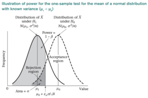
– Rosner, B. Fundamentals of Biostatistics (7th ed.), p. 222.
When we design an experiment, we usually set values for alpha, beta (and power). But we also need to define what change we expect to see between the two groups. What change will matter in this particular case? This is called practical significance or also known as the desired effect size. These three factors: alpha, power, and effect size are directly related to sample size. The relationship between them is complex and interdependent. It’s a very important concept to understand.
Sample Size and Its Importance
The sample size plays a critical role in hypothesis testing. It affects the values of alpha, beta, and power. Increasing the sample size generally decreases both alpha and beta, while increasing power. This is because a larger sample size provides more data and reduces the sampling error. This makes it easier to detect a true effect if one exists. As a result, a larger sample size generally leads to a more accurate estimation of the population parameters. This in turn increases the power of the test.
On the other hand, decreasing the sample size generally increases both alpha and beta, while decreasing power. This is because with a smaller sample size, there is a higher chance of random variation affecting the results. This can lead to a false positive or false negative conclusion. As a result, a smaller sample size can decrease the accuracy of the estimation. This in turn decreases the power of the test.
The effect size directly affects the sample size. A larger effect size generally requires a smaller sample size to achieve the same level of power. Conversely, a smaller effect size will require a larger sample size to achieve the same level of power. The effect size can be thought of as the magnitude of the difference between the groups being compared. It is typically measured using standardized effect size measures such as Cohen’s d.
Alpha, power and effect size in A/B Testing
Graph of alpha, beta and power in the case of a small sample size vs large sample size for a the same effect size of 0.02:
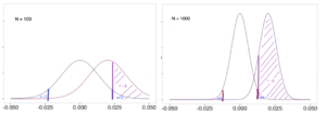
Note that if we increase the effect size, for example from 0.02 to 0.1, the center of the distributions would be further apart, since the distance between 0 (the case of the null hypothesis where the groups have the same metric) and 0.1 is much greater than between 0 and 0.02, we would have less error, and we would need less data. This means that a larger effect size can lead to more statistically significant results with a smaller sample size.
It is also important to consider the practical significance of the effect size, as a very small effect size may not be meaningful, even if it is statistically significant. The effect size indicates what difference is relevant in business terms and quantifies what change is important to occur. It depends on the experiment being conducted. It is not the same in a medical context, for example, where we are testing whether a new drug will improve patient outcomes, as it is in evaluating whether changing a feature on a website will improve conversions. In the former case, a 5-10% difference can be considered practically significant, because if the change is very small, it is not worth the cost of introducing a new drug. On the other hand, in the latter case, a 1-2% difference can be relevant when we are talking about thousands of users, making it worthwhile to implement the change.
Overall, the relationship between effect size and sample size highlights the importance of carefully considering the research question and the magnitude of the effect being studied when designing experiments.
How to Choose the Sample Size in A/B Testing?
Determining the sample size is one of the most important steps in designing an A/B test. A sample size that is too small can lead to inconclusive results, while a sample size that is too large can waste resources. Therefore, it is important to choose an appropriate sample size for your A/B test.
As previously mentioned, the sample size required for a hypothesis test depends on various factors, including the size of the effect that is expected to be observed, the desired level of significance, the power of the test, the type of statistical test used, and the variability of the data.
First let’s import the library
import statsmodels.stats.api as sms
Significance level:
This is what we previously called alpha, a significance level is typically set at a pre-determined value (such as 0.05 or 0.01), and is used in hypothesis testing to determine whether to reject or fail to reject the null hypothesis.
alpha = 0.05
Practical significance:
Also known as the size of the effect, If our variable is a proportion and we want to observe if our CTR goes from 0.10 to 0.15, we will use the function proportion_effectsize to obtain the corresponding value.
effect_size = sms.proportion_effectsize(0.10, 0.15)
If our variable is a mean, and we want to see if it changes by 5%, we also have to take into account the standard deviation of the distribution from which we are estimating, this deviation can be calculated based on a sample of the population under study.
std= 0.53
effect_size = 0.05/std
Power:
A value of 0.8 is commonly set as the threshold for power.
power = 0.8
Finally we calculate the required sample size as:
required_n = sms.NormalIndPower().solve_power(
            effect_size,
            power=power,
            alpha=alpha)
Factors Affecting the Sample Size
- As the standard deviation increases, the required sample size also increases.
- Lowering the significance level (decreasing α) will lead to an increase in the sample size.
- If the required power (1 − β) increases, this will also drive an increase in the sample size.
- The absolute distance between the null and alternative means (|µ0 − µ1| -> effect size) increasing causes a decrease in the sample size.
The success of an A/B test depends on the quality of the experiment design, the accuracy of the data collected, and the rigor of the statistical analysis. So, make sure you carefully plan and execute each step of the test to achieve meaningful results that can inform your decision-making.
Hypothesis test
Once we have collected all the samples that we define as necessary to carry out the test, we are going to proceed to execute it. For this there are different options:
Hypothesis testing can be performed using both parametric methods, which assume an underlying distribution, such as z-test and t-test, or non-parametric methods, which do not make any assumptions about the distributions, such as Fisher’s Exact test, Chi-Squared test, or Wilcoxon Rank Sum/Mann Whitney test. Note that the choice between parametric or non-parametric methods depends on the data being analyzed and the assumptions we can make about the underlying population. For example, we may use parametric methods for normally distributed data, while non-parametric methods can be employed for non-normal or skewed data. Always carefully consider the choice of method to ensure the validity and reliability of the results.
Two sample Z-test
Usually the hypothesis tests to be carried out in ab testing comprise a sample size greater than 30, so we are going to execute z-type tests assuming a normal distribution.
Z test for proportions
Let’s suppose that for the example analyzed, we obtained the necessary samples for control and treatment, with sizes of 10.072 and 9.886, respectively. In the control group, 974 clicks were made, and in the treatment group, 1.242 clicks were recorded. Let’s perform the test for this situation:
from statsmodels.stats.proportion import proportions_ztest, confint_proportions_2indep

X_con = 974 #clicks control
N_con = 10072 #impressions control
X_exp =  1242 #clicks experimental
N_exp = 9886 #impressions experimetal

successes = [X_con, X_exp]
nobs = [N_con, N_exp]

z_stat, pval = proportions_ztest(successes, nobs=nobs)
low_c, up_c = confint_proportions_2indep(X_exp, N_exp, X_con, N_con, compare='diff', alpha=alpha)

print(f'z statistic: {z_stat:.2f}')
print(f'p-value: {pval:.3f}')
print(f'ci 95% for difference: [{low_c:.3f}, {up_c:.3f}]')
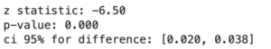
The p-value is less than the predefined alpha of 0.05, which means that we can reject the null hypothesis and conclude that there is a significant difference between the two groups. A confidence interval of [0.02, 0.038] for the difference between the two CTRs also suggests that the true difference between the two CTRs falls within this range with a certain level of confidence (95%). Since the interval does not include 0 (and therefore the p-value is very close to zero) which is the hypothesized value for no difference between the groups, we can conclude that there is a statistically significant difference. In other words, we reject the null hypothesis that the CTRs are equal and instead accept the alternative hypothesis that the CTRs are different.
Z test for means
If instead our metric is a continuous variable, we’ll simulate two groups of size 60, where the metric can take random values from a normal distribution of mean 10 and standard deviation 4 for both groups, and run the test:
from statsmodels.stats.weightstats import ztest, zconfint

N_con = 60
N_exp = 60
X_con = np.random.normal(10, 4, size =N_con)
X_exp = np.random.normal(10, 4, size = N_exp)

z_stat, pval = ztest(X_con, X_exp)
low_c, up_c = zconfint(X_con, X_exp, alpha=alpha)

print(f'z statistic: {z_stat:.2f}')
print(f'p-value: {pval:.3f}')
print(f'ci 95% for difference: [{low_c:.3f}, {up_c:.3f}]')
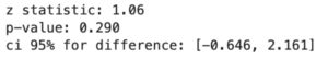
In this case, since the p-value is greater than alpha and the confidence intervals include zero, we conclude that there is no significant difference between the means and accept the null hypothesis.
A/B testing with Bootstrapping
Bootstraping is a useful technique in A/B testing when the sample size is small or when the underlying distribution of the data is unknown. Bootstraping involves generating multiple random samples with replacement from the original sample to create an empirical distribution of the sample statistics. It can help to estimate the sampling distribution of the test statistic without relying on the assumptions of normality and equal variance required by traditional parametric methods.
def test_bootstrap(trmt, ctrl, N=1000):
    metric_diffs = []
    mean_control = []
    mean_treatment = []

    # Repeat the experiment N times
    for _ in range(N):
        data_ctrl = ctrl.sample(frac=1.0, replace=True)
        data_trmt = trmt.sample(frac=1.0, replace=True)

        # Measure mean values
        metric_mean_ctrl = data_ctrl.mean()
        metric_mean_trmt = data_trmt.mean()

        # Measure difference of the means
        observed_diff = metric_mean_trmt - metric_mean_ctrl
        metric_diffs.append(observed_diff)
        mean_control.append(metric_mean_ctrl)
        mean_treatment.append(metric_mean_trmt)

    obs_diff = trmt.mean() - ctrl.mean()
    standard_dev = np.array(metric_diffs).std()
    h_ = np.random.normal(0, standard_dev, np.array(metric_diffs).shape)
    p_val = np.logical_or(np.array(h_) >= obs_diff, np.array(h_) <= -obs_diff).mean()
    exp_dif = np.array(metric_diffs).mean()

    left_i, right_i = np.percentile(np.array(metric_diffs), [5,95])
    left_i, right_i = round(left_i,3), round(right_i,3)
    exp_dif = round(exp_dif, 3)

    print(f'p-value (trmt==ctrl): {p_val:.3f}')
    print(f'expected dif (trmt-ctrl): {exp_dif:.2f}')
    print(f'ci 95% for difference: [{left_i:.3f}, {right_i:.3f}]')

    # Plot distribution of the means for control and treatment
    boot_gr = pd.DataFrame({"control": mean_control, "treatment": mean_treatment})
    boot_gr.plot(kind='kde')
    plt.show()

    # We can also see the difference as a dist plot here
    boot_gr = pd.DataFrame({"equal_means": h_, "diff_means": metric_diffs})
    boot_gr.plot(kind='kde')
    plt.show()
n = 100
X_ctrl = np.random.normal(4.5,3,n)
X_trmt = np.random.normal(5,3,n)

test_bootstrap(pd.Series(X_trmt), pd.Series(X_ctrl))
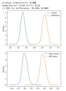
In the simulated example, we randomly generate two normal distributions, one with a mean of 4.5 and the other with a mean of 5, with the same standard deviation of 3. The first plot shows both distributions, and we can see that there is a real difference between them. In the second plot, we observe two distributions. One distribution is centered at zero, corresponding to the null hypothesis if the means were equal. The orange distribution represents the difference between treatment and control obtained by bootstrapping. As shown in the plot, there is a difference of 0.5. The calculated p-value and confidence intervals support the decision to reject the null hypothesis
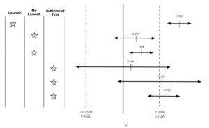
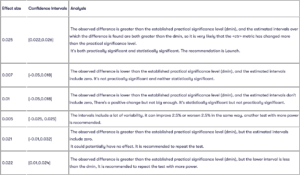
Possible outcomes: confidence interval cases
When we calculate the difference between the two groups and elaborate the confidence intervals on it, we can find different results. The following graph shows the confidence intervals with respect to a practical significance level (dmin) established at 0.02.
Conclusions
In conclusion, A/B testing is a powerful tool for businesses and individuals who want to optimize their digital products and marketing campaigns. By using statistical methods to test different variables and designs, we can gain valuable insights into what works and what doesn’t. It’s important to remember that A/B testing is not a one-time fix, but an ongoing process that requires continuous testing and iteration. By carefully choosing our sample sizes, using appropriate statistical tests, and considering the limitations and assumptions of our experiments, we can make data-driven decisions that ultimately lead to improved user experiences, higher conversions, and greater success.
If you are interested in knowing more about data science and machine learning, feel free to check out our in-depth articles on: https://blog.marvik.ai/
References
– Rosner, B. Fundamentals of Biostatistics (7th ed.)
– Udacity course: A/B testing. https://www.udacity.com/course/ab-testing–ud257
– Tatev Karen Aslanyan, Complete Guide to A/B Testing Design, Implementation and Pitfalls. https://towardsdatascience.com/simple-and-complet-guide-to-a-b-testing-c34154d0ce5a

