Reinforcement learning: AI meets Pavlov’s dog

Introduction

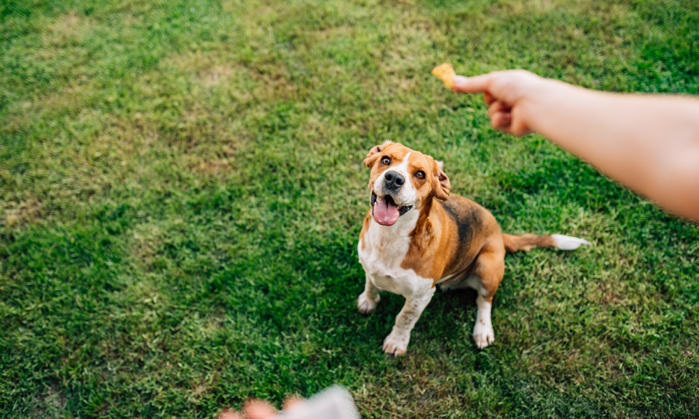
Ever heard of Pavlov’s dog? In 1897 Ivan Pavlov, a russian physiologist, published his findings on conditioned behavior, that demonstrated how dogs could be conditioned to associate an unconditioned stimulus (food) with a neutral stimulus (bell), leading to a conditioned response (salivation) triggered by the bell alone. 

The idea behind this experiment is that the dog could be conditioned to behave in a certain way according to a series of rewards or punishments it received, which is the central idea behind reinforcement learning.  Both Pavlov’s dog and reinforcement learning systems showcase the power of conditioning and the ability to adapt behaviors based on reinforcement signals.

In this blog we’re going to explore the basics of reinforcement learning, learning top down. This blog is aimed at readers with some understanding of calculus and algebra, but you don’t need to be an expert to follow through. 

What is reinforcement learning?

Reinforcement learning is a mathematical approach to learning by trial and error, and it seeks to emulate one of the ways by which animals learn.  Imagine you get a small puppy who you want to teach tricks to. They will learn to do these tricks by trial and error, falling down, occasionally bumping into furniture (negative feedback) but also being praised by you and rewarded treats when they manage to make progress (positive feedback). Over many attempts, they will progressively learn how to perform the tricks better and eventually on their own, without the need for the treats. This is the phenomenon reinforcement learning tries to learn from.  

The main idea behind reinforcement learning is that an agent (a model, but in our previous example, the puppy) will learn from the environment (in this case, you and your surroundings) by interacting with it (attempting the trick, falling) and receiving feedback (being praised, given treats) each time they interact in a different manner. Each interaction is known as action (the movement the dog makes) and the received feedback is given by a reward function (the treat we give him or deny him), that can be positive or negative in case an action has a negative consequence.

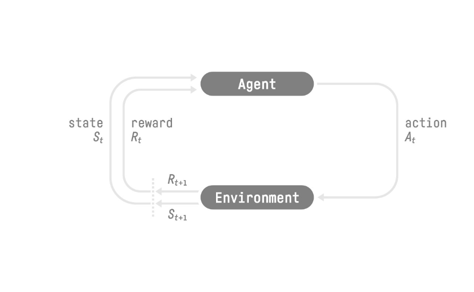
In the figure above St, At, Rt, refer to the state, action and reward at time t. In the puppy example, the state would refer to whatever position the dog is in at time t, the action which movement it is performing and the reward to whether or not you are going to feed him a treat. 

Action and State Space

Reinforcement learning scenarios have an associated state or observation space, that is, a complete or partial description of the environment. For example, in the case of an agent learning to play chess, the agent has a complete description of the environment since it knows the position of every other piece on the board at a given step. Complete descriptions of the environment readily available are not the rule and partial descriptions are known as observations. 

These types of scenarios also have an associated action space, that is, the set of all possible actions an agent can perform. This action space can either be discrete, like in the case of chess playing where there are a set of possible actions a given piece can take, or continuous, like the action space while driving a car.

Reward model

The reward model is the core of reinforcement learning since it provides the agent the feedback it needs to learn. The reward of a trajectory (in chess, for example, a trajectory could simply mean a series of sequential actions the agent takes) is given by the sum of the discounted rewards at each timestep:

R(τ)=r(t+1) +ɣr(t+2)+…+ɣk-1r(t+k)

R is the cumulative reward function over the whole trajectory τ and it is made up of the reward obtained at each timestep 1 through k necessary to complete τ. 

ɣ is known as the discount rate and its introduction is needed since rewards further away from the current state are less likely to happen than those closer to the current state. Think of it this way: if you’re playing chess and planning a series of 4 moves to take your adversary’s queen, he could potentially move his queen before you reach it or take one of your pieces which was key to your strategy and thus you wouldn’t be able to complete your move. Rewards further away from the current state need to be discounted since they are less likely to happen than those closer to the state.

Types of reinforcement learning: 

But how do these agents learn from the environment? How do they know which action to take at any given state in order to maximize their cumulative reward? Well,  this is where policy comes into play. The policy of a reinforcement learning task, noted π, is the model that tells the agent how to behave at any given state. This is the function we aim to learn in order to find the optimal policy π that maximizes the cumulative reward of the agent. 

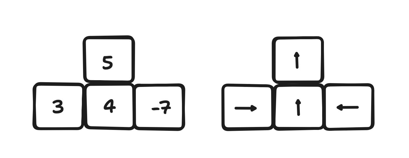
There are two main approaches to finding π: policy based methods and value based methods.  On the one hand, value based methods aim to learn a value function that maps the state to the expected value of being at that state. The policy used in this scenario is simply to take the action that leads to the state with the highest value. 

On the other hand, policy based methods aim to learn the function π directly, that is, a mapping of what action is best to take in each given state. This policy can either be deterministic (for a given state S, the optimal action is always A) or stochastic, yielding a probability distribution over all actions at each state. 

Policy gradients

One of the main approaches to stochastic policy learning is the use of a neural network whose parameters are tuned using gradient descent, a process which is called policy gradients. The simplest approach taken is policy gradient, which simply updates the parameters of the policy by a learning rule much like the one used in supervised learning:

𝚹 ← 𝚹 + ɑ∇𝚹 J(𝚹)

Where 𝚹 is the vector with all the parameters that make up the policy, ɑ is a preset learning rate and ∇𝚹 J(𝚹) is the gradient of the cost function J (the function that measures how far the policy is from the optimal response) with respect to the parameters. This structure resembles steepest descent of a neural network in a supervised learning problem, and the update rule is also very similar given that, generally speaking, policies are approximated using neural networks. 

But policy gradient suffers from major drawbacks:

• It is a Monte Carlo learning approach (which means averaging the reward the agent gets through a whole episode), taking into account the full reward trajectory (a sample), which often suffer from high variance which leads to convergence issues.  
• Samples are only used once, once the policy is updated, the new policy is used to sample a new trajectory, which is an expensive process
• Choosing the right learning rate ɑ is difficult and the system suffers from both vanishing and exploding gradients, which leads to convergence being very sample dependent

Proximal Policy Optimization

In order to tackle these and other drawbacks of policy gradients, several other algorithms have been explored. The current state of the art models are those derived from Proximal Policy Optimization (PPO), a paper published back in 2017. The math behind it is challenging and exceeds the scope of this review, but essentially, PPO improves upon policy gradient in two major ways:

• PPO introduces a target divergence term, which penalizes cases in which the updated policy produces results that differ too much from past samples. We would like our policy to return results within a certain neighborhood, so that answers are similar from one step to the following. 
• Since this divergence caps the difference between two consecutive samples this means that updates to the policy are small and thus, samples can be reused more than once to update the policy.

Reinforcement Learning From Human Feedback

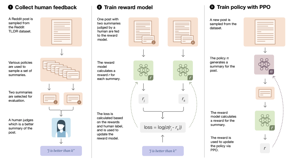
At an abstract level we have been through a few of the approaches used in reinforcement learning. But how exactly do you train an agent to solve a real problem given we do not know the reward value for any given state in the state space? Well, the most used approach at present day is reinforcement learning from human feedback (RLHF). 

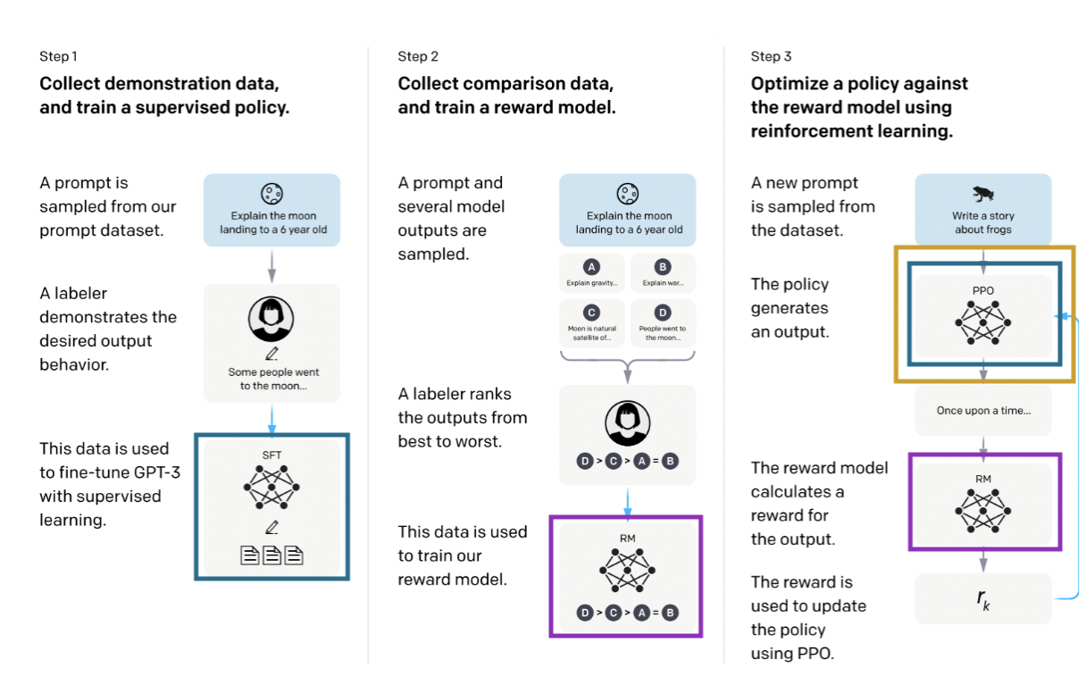
The process has three steps. Step 1 is to train a supervised policy (in blue in the diagram above), which simply means training a neural network, here policy and neural network are synonyms. Then  in step 2, several outputs of the policy are ranked from best to worst by labelers (other approaches include awarding each output a score) and this input is used in step 3 to train what we call a reward model (in purple), another neural network which will take an output from a policy and award it a reward. This reward model is then used to update the policy using PPO (in yellow), where for each training step the output of the PPO is scored by the reward model.

This training modality of first training a supervised policy that is then fine tuned using reinforcement learning has been lately widely used, its most famous example being ChatGPT. Other areas where PPO is widely used are stock trading as well as robotics.

Case Study: Writing positive movie reviews 

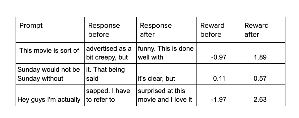
One of the most complete repositories to finetune models using reinforcement learning is TRL, which can be used to finetune transformers. We tried it out by fine tuning GPT-2 to produce positive movie reviews, using IMDB’s dataset. We used a pre-trained DistilBERT model to perform sentiment analysis over reviews and used it as our reward model. 

Two copies of GPT-2 were used: one frozen, being only trained using supervised learning, and one whose weights were changed at each iteration in order to compare past and current behavior.

In the diagram, Prompt simply refers to an incomplete description that GPT needs to complete. Performing sentiment analysis over the two outputs, the reward of the current output of the fine tuned model is computed and with that its weights are modified. An example of the performance of the model before and after fine tuning is shown below.

Conclusions

In this article we have gone through the basics of reinforcement learning, building from key concepts like state space, action space and reward model up to how to use human feedback to finetune language models. We mentioned a few areas in which reinforcement learning is particularly used and we went through one application, writing positive reviews for movies. Reinforcement learning from human feedback techniques are currently all the rage in the fine tuning phase of large language models, but can be used in a broad series of scenarios where a reward function can be constructed in order to guide the learning process.  

References

Sutton, R., Barto, A., ‘Reinforcement Learning: An Introduction’, 2018

Schulman, J., et al, ‘Proximal Policy Optimization Algorithms’, 2017

Ouyang, L. , et al, ‘Training language models to follow instructions with human feedback’, 2022