First steps in implementing a multi-head architecture
By Sofía Pérez
Intro
In life, we are constantly dealing with several situations at the same time. This comes naturally to us, and most times we are not even aware of the fact that we are doing it. For instance, while driving a car, we must certainly be aware of different things and make real-time decisions accordingly: detecting pedestrians crossing the street, keeping track of other cars’ maneuvers, detecting lane markings, reading traffic signs, among other things.
Now, how can we translate this into a deep-learning solution? Do we need to develop separate models to tackle each task? Or can we benefit from the fact that there is a common starting point? This is one of the main topics that was referred to during Tesla’s AI Day 2021 talk, which encouraged our research. In this keynote, Tesla introduced for the first time the concept of using a multi-head architecture (named Hydra Net) applied to autonomous driving. Throughout our investigation, it came to our attention that this novel approach of multi-task deep learning has not yet been heavily exploited and that there is not much work done in this aspect. In fact, most implementations focus on specific single tasks rather than tackling the problem as a whole.
The aim of this post is to present an approach to fully recreate the concept of multi-head networks introduced by Tesla and appreciate its benefits. We will focus on solving two specific tasks: lane segmentation and object detection in driving scenarios. We consider that both functions are key to successfully deploying an autonomous driving solution. Lane segmentation implies detecting all possible drivable areas. It requires the model to be able to detect free lanes, opposite driving sends, side walks, parking entrances, among others.
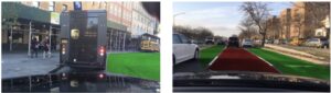
Images obtained using UNet segmentation model
On the other hand, object detection involves being able to detect all visible objects and classify them accordingly. In terms of driving, this generally includes detecting other cars, traffic signs, traffic lights, pedestrians, among others. The fact that objects might have varying sizes and shapes, and the possibility of partial occlusion compose some of the challenges of this specific task.
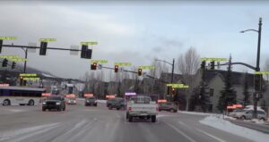
Image obtained using YOLOv7 model
Both concepts, lane segmentation and object detection, have been deeply studied separately during past years. Most common solutions involve using a Mask R-CNN architecture for image segmentation and YOLO (in its different flavors) for object detection. However, these tasks are not usually addressed jointly. In terms of autonomous driving solutions, computing capacities are usually bounded, as the model is required to run inside the vehicle. This shortcoming makes the idea of running the model as a whole even more tempting.
Multi-head architecture
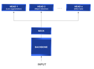
A multi-head network usually consists of the following modules:
- Backbone: It is a common feature extraction network that, as its name implies, is used to extract relevant information from the input data and generate its corresponding feature map.
- Neck: Located between the backbone and the heads, this module is usually used to extract further information and more elaborate features using pyramidal techniques.
- Head: This type of module is deployed to solve more specific tasks using the feature maps generated by the backbone and neck modules.
The following diagram gives you a further understanding of the general structure of a multi-head network typical architecture.
What makes this type of architecture so appealing is its capability of feature sharing between the different heads. This implies a direct reduction in repetitive tasks, convolution calculations, memory, and the number of parameters used. It’s especially efficient at test time.
In terms of autonomous driving, the heads are designed for different purposes such as lane segmentation, traffic sign detection and tracking, among many others. But, for what is worth, this concept can be abstracted and applied to any other scenario which needs to tackle different tasks simultaneously and can benefit from sharing a common backbone.
The rest of this post is organized as follows. First, we will introduce our model’s architecture, deep diving into each of its components, with special focus on the interconnection of each block. Next, we will present some of the results obtained in this proof of concept, which turned out to be very promising. Finally, we will discuss possible next steps and improvements.
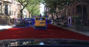
Image obtained using our Multi-Head model
Our model
As we previously mentioned our main goal was to develop a multi-head model capable of performing two tasks: object detection and lane segmentation.
Instead of jumping right into current state-of-the-art models for each subject and figuring out how to join their complex architecture, we opted to take a few steps back. Our approach focuses on keeping things as simple as possible at first, to gain a full understanding of the architecture interconnections.
Our backbone consists of a ResNet34 network which is then attached to a classical Feature Pyramid Network (FPN) block. The different outputs of the pyramid are then connected to the segmentation and object detection heads, which are based on the UNet and RetinaNet models respectively. Now, let’s review how these components were built, shall we?
Backbone
The backbone module consists of a feature extraction network. To this end, ResNet seemed to be a good starting point and could be easily connected to a vanilla FPN network, without adding further complexities to the model.
ResNet
ResNets are a type of convolutional neural network capable of increasing depth while dealing very well with the vanishing gradient problem. The core idea behind this is to apply shortcut connections that skip one or more layers.
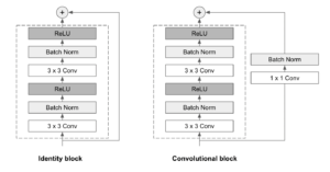
ResNets are made up of a series of residual blocks, also referred to as ResBlocks. Each ResBlock consists of two 3×3 convolutional layers, each one followed by a batch normalization layer and a ReLU activation function. A skip connection is then used to add the input to the output of the block. Two types of the block are used, depending on whether the input and the output dimensions are the same or not:
- Identity block: When the input and output dimensions are the same, the skip connection joins the input directly to the output of the ResBlock, and adds them up. No further modifications are needed.
- Convolutional block: When the input and output dimensions do not match, a 1×1 convolutional layer followed by a batch normalization layer is applied in the skip connection path.
ResNets can have variable sizes and layers. In our implementation, we’ve chosen to use a ResNet34 (34 layers) architecture, which seemed to be the wiser choice in line with keeping things as simple as possible.
FPN
Feature Pyramid Networks (FPN) are intended to help detect objects in different scales, generating multiple feature map layers. It is composed of two pathways: bottom-up and top-down.
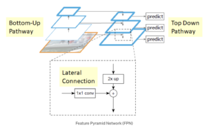
The bottom-up pathway is the usual convolutional network for feature extraction. As we go up, the spatial resolution decreases but the semantic value increases. In the original paper, this was built using a ResNet.
The top-down pathway constructs higher-resolution layers from a semantic rich layer. Lateral connections are added between reconstructed layers and the corresponding feature maps to help the detector to predict the location better. It also acts as a skip connection to make training easier.
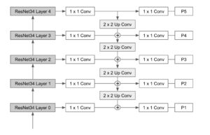
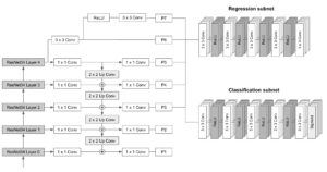
The following diagram depicts the final backbone architecture combining ResNet and FPN levels.
Segmentation Head
Aligned with developing a simple approach, we decided to base the segmentation head on a classical UNet model which has proven to be useful for this type of problem.
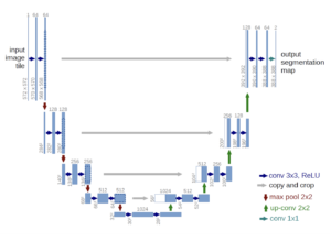
The UNet architecture is fully convolutional and basically consists of three parts:
- Contracting Path (Encoder): It consists of 4 blocks. Each one applies a 3×3 convolution + ReLU combo twice (“Double-convolution”), followed by a 2×2 MaxPool with stride 2 for downsampling. At each downsampling step, we double the number of feature channels.
- Bottleneck: It’s a 3×3 convolution + ReLU combo repeated twice. It acts as a bridge between the encoder and decoder pathways.
- Expansive Path (Decoder): It consists of 4 blocks. Each one applies an upsampling of the feature map followed by a 2×2 convolution (“Up-convolution”), then followed by a concatenation with the correspondingly cropped feature map from the contracting path, and two 3×3 convolution + ReLU combo (“Double-convolution”). The concatenation step helps prevent spatial information loss due to downsampling. At the final layer, a 1×1 convolution is used to map each 64-component feature vector to the desired number of classes.
Detection Head
In terms of one stage object detectors, the RetinaNet model has proven to work very well on small objects. What’s more, in essence, its backbone consists of an FPN built on top of a ResNet which aligns perfectly with ours. Thus, it seemed the best way to go for building our detection head.
RetinaNet was introduced by the Facebook AI research team in 2017. Its design aimed to tackle dense and small object detection problems by introducing two improvements to classical object detection models:
- Incorporating Feature Pyramid Networks (FPN) into the backbone.
- Using the Focal Loss function for the classification subnet loss.
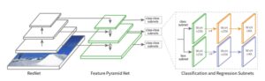
RetinaNet’s architecture consists of the following:
- Backbone: A fully convolutional backbone responsible for computing the feature map over the entire image at different scales. For RetinaNet, the FPN is built on top of ResNet architecture. The pyramid has 5 levels, P3 to P7, covering the following resolutions: [23, 24, 25, 26, 27].
- Classification subnet: A fully convolutional network attached to each pyramid level that aims to predict the probability of an object being present at each spatial location for each anchor box and object class. It consists of applying four 3×3 convolutional layers with M filters followed by ReLU activations, with M being the number of channels at each pyramid level. Finally, it applies another 3×3 convolutional layer with CxA filters, with C being the number of target classes and A the number of anchor boxes (9 by default), followed by sigmoid activations that are used to get the final classification score.
- Regression subnet: A fully convolutional network attached to each pyramid level that runs in parallel to the classification subnet. Its purpose is to regress the offset from each anchor box to a nearby object (if one exists). The design of the box regression subnet is practically identical to the classification network, the only difference is that the last 3×3 convolutional has 4*A filters, with A being the number of anchor boxes (9 by default). In other words, for each of the A anchor boxes per spatial location, 4 outputs are predicted, which represent the relative offset between the anchor and the ground truth box).
The following scheme illustrates RetinaNet’s architecture and the interconnections between its different modules:
Anchor boxes
RetinaNet uses anchor boxes with fixed sizes as a prior to predicting the actual bounding box of each object. The anchors have areas ranging from 32×32 to 512×512 on all pyramid levels (P3 to P7). Moreover, to improve coverage three aspect ratios [1:2, 1:1, 2:1] and scales [20, 21/3, 22/3] are incorporated into the design, resulting in a total of 9 anchors per level per spatial location. With this setup, the anchors manage to cover the scale range from 32 to 813 pixels relative to the input image.
For each anchor, an intersection-over-union (IoU) score is calculated. If the IoU score is greater or equal to 0.5 then the anchor is assigned to a ground-truth object and is factored into the loss function. If the IoU is between 0 and 0.4 then it is considered as background. Finally, if the score lies between 0.4 and 0.5 it is ignored.
At each pyramid layer thousands of anchor boxes are generated (9 per each spatial location in the image), but only a few will actually contain objects. This vast number of easy negatives can overwhelm the model, thus Focal Loss was introduced to prevent this. Basically, Focal Loss reshapes the classical Cross-Entropy Loss (CE) by incorporating a dynamical scaling factor that decays to zero as the confidence in the correct class increases. In other words, this scaling factor automatically down-weights the contribution of the easy examples such as easy negatives and rapidly focuses on improving the hard ones.
A few things to keep in mind…
RetinaNet uses fixed anchor sizes which may need to be tuned accordingly. Default size values are [32, 54, 128, 256, 512] i.e. objects smaller than 32 by 32 pixels will not be detected by the model. Taking this factor into account, to accomplish an adequate design of the anchor boxes, it is a good practice to review the following points:
- Identify the smallest and largest objects that are to be detected.
- Identify the different shapes that a box can take, meaning the possible ratios between the height and width of a box.
Putting all together
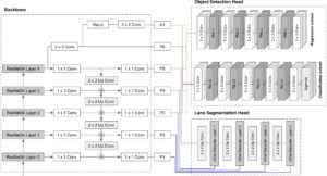
Now that we have reviewed each component separately, in this section we’ll walk you through the process of connecting all the pieces. As we’ve introduced earlier, our backbone is the same as RetinaNet’s, so we will only need to focus on how to connect the segmentation head to our backbone.
Taking a close look into UNet’s architecture, one can realize that the encoder path can easily be substituted for our ResNet + FPN backbone. To do so, layers P1 to P5 of the pyramid network are concatenated to the inputs of Unet’s decoder blocks.
The following diagram intends to describe the model’s final architecture.
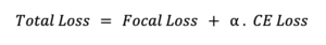
In order to train the final model, an adequate loss function must be defined. We’ve addressed this requirement by performing a weighted sum that combines the losses of each head: Cross Entropy for the segmentation head and Focal Loss for the object detection head.
Our Results
We’ve trained our model using the Berkeley Deep Drive dataset (BDD100k) and we were able to obtain very encouraging results regardless of only having used 5 epochs for training. Some of the results obtained on the test set are shown in the images below.
As you can see, the model not only accomplishes segmentation of the drivable lanes but also manages to detect different objects of varying sizes and classes present in the images.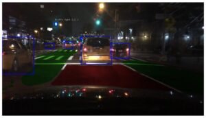
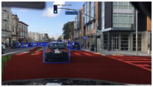
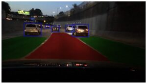
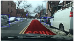
To further validate the model’s performance, we’ve also run it on some images of Montevideo city streets, obtaining pretty awesome results. As this images are outside of the BDD100k dataset, we’ve demonstrated that our model is also capable of generalizing very well.
Conclusions & Next steps
We did it! We were able to successfully implement a simple yet powerful two-headed model for object detection and image segmentation. The results achieved with this approach have proven to be quite promising, reaffirming the advantages of implementing the multi-head approach. Yet, the simplicity used in the architecture has given us a deeper understanding of the solution as a whole.
As for possible next steps, some of the following might be good starting points:
- Improving anchor selection in RetinaNet by implementing a clustering algorithm, e.g k-means, to determine the appropriate anchor sizes based on the training data.
- Dive deeper into fine-tuning loss ponderation.
- Substituting our vanilla version of FPN for an Extended FPN. In this way, we can incorporate the feature map of the P2 level of the pyramid without jeopardizing real-time performance.
- Substitute ResNet34 for deeper versions such as ResNet101 or ResNet 50 to achieve higher accuracy.
We hope you’ve enjoyed this post. Stay tuned for more!
References:
- Deep Residual Learning for Image Recognition
- Feature Pyramid Networks for Object Detection
- U-Net: Convolutional Networks for Biomedical Image Segmentation
- Anchor Boxes — The key to quality object detection
- Focal Loss for Dense Object Detection
- Berkeley Deep Drive dataset (BDD100k)

