Multi-image similarity: an approach for a recurring problem
By Julián Peña and Sebastián Portela
Motivation
Images are everywhere. You may know the expression ‘an image is worth a thousand words’. The amount of information a single look at an image can give us is huge, and we can process it in as little as 13 milliseconds!
As human beings, we think in terms of images and that’s why we are captivated by movies, television and websites. We have become a visually oriented society. People are used to seeing and responding to images and this has given rise to hundreds of image-based applications. Image restoration or generation (such as dall.e), defect detection, content-based recommendation and online image searching are some examples of this vast universe of implementations.
Many of these applications rely on image similarity algorithms to perform their main task. We can think of a semi-supervised model for dataset construction. With this model, new images can be automatically labeled by computing their similarity with every other image of a labeled dataset.
As the reader will see throughout the article, image comparison is not a difficult task, at least, not when we are comparing one image to another. The challenge we want to address here is the comparison between sets of images. A set of images of an object has certainly more information than a single image and that’s why this challenge is attractive.
It is clear that this extension turns the problem from an almost trivial one to a quite complex one. We’ll try to guide you step by step on how we are dealing with it.
Problem statement
Our main goal is to reach an appropriate metric to compare sets of images. This was first studied in the context of e-commerce, with the aim of recommending similar products from which multiple images are available.
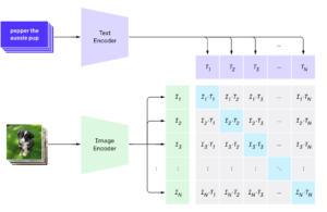
In order to compare images and find similarities we will take advantage of how Convolutional Neural Networks (CNNs) work and are able to classify images in different categories. From the usual cat/dog discrimination to the image-net dataset that has 1.000 different categories.
If you feed an image to a trained CNN, the image will be converted into a vector (embedding) that retains the main features of the image. This vector is used by the last layer of the CNN to classify the image into a category. For example, to tell if the image was a dog or a cat. It is possible to see that all vectors from a certain category are grouped together in the multidimensional space.
We will use this characteristic to find similarities between any images. We will feed two different images to a CNN, extract their corresponding vectors and, if these two vectors are close to each other, we will conclude that the two original images are similar. To measure the distance between two vectors we can calculate their cosine similarity, and we will refer to (1 – cosine similarity) as the similarity score.
There are many pre-trained traditional CNNs we could use to convert images to vectors (VGGs, Resnets, Efficient-nets). We decided to try the Hugging Face implementation of the CLIP model. CLIP was envisioned mainly to find image-text similarity but we can perfectly use it for our image-image similarity purpose. CLIP has also shown state-of-the-art performance in many classification tasks with zero-shot predictions without any fine-tuning specific training.
Simplest case: Single-image
Before diving into deeper waters we will try to find similar images within a shoe dataset, extracting data from the 44K Fashion dataset. It has 315 different shoes with different characteristics. The pipeline is the following:
- Resize, crop and pad images to a 240×180 resolution each of the 315 images.
- Transform images to 512 dimensional vectors using CLIP’s image encoder.
- Calculate a (315×315) distance matrix between all image vectors.
- Extract the nearest images for any given shoe.
In the images below we can see 4 examples. For each shoe we ask the model to give us the 3 nearest images within the dataset. We can visually confirm that it’s doing a good job, separating the sport shoes, from the formal and casual ones. It also correctly separates two different types of casual shoes (two last sets of images)
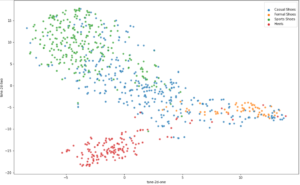
Plotting our image vectors
As anticipated, we can see how the different categories of the shoe dataset tend to cluster together. An interesting tool for visualizing vectors is t-SNE. We reduced the vectors to only two dimensions for visualization purposes. We can also see that casual shoes intersect with formal and sport shoes and that makes complete sense. Remember that our vectors have 512 dimensions so it’s quite impressive that with just two dimensions we can achieve this level of clustering.
Some spice: Ordered multi-image
That was quite simple, but remember that in reality we usually have to face more general scenarios and, as you may have noticed, we generally have more than one image per article when browsing e-commerce websites. This opens a whole new range of opportunities but also some obstacles.
The simplest situation in this multi-image universe would be the one where each article has the same amount of images, taken under the same rules (angle, background, article-background ratio, etc.) and equally ordered.
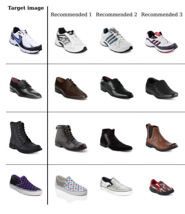
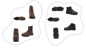
Here we have a target article for which we’ll find the most similar article from a subset of three other candidates. There are four images for each article, perfectly tagged as right, top, back and front. For each tag, there’s also the similarity score computed for each candidate related to the target article.
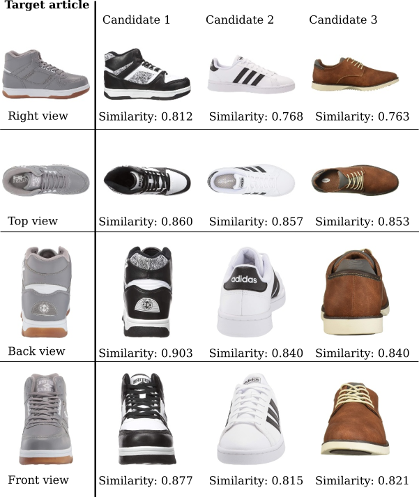
Well, it looks simple enough. We could just average the similarities of each candidate and the k articles with the highest similarity should be the recommended ones. In this case , with k=1, the Candidate 1 would be the recommended one related to the Target article.
The real challenge: Generic multi-image
So far we had a pretty comfortable scenario where an ordered set of n images of each object was available (with the particular case of n=1). This configuration allowed us to compare the images of each set in order and get an average similarity. But what happens when the images are not ordered at all? What if the size of each set is different? This is how we handled it:
Recursive matching
The idea behind this approach is to get the best match in each iteration, discarding the images that were already matched.
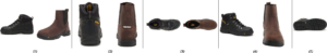
Let’s suppose we want to get the similarity of a boot with 4 images relative to another boot with 5 images. Each set is independent and not all the pictures are taken from the same angle.
The first step is to compare all the images on one side to the images on the other. By doing this, we get a 4×5 matrix with the similarity score of each pair of images:
| cat_black_1 | cat_black_2 | cat_black_3 | cat_black_4 | cat_black_5 | |
| cat_brown_1 | 0.837 (3) | 0.835 | 0.747 | 0.703 | 0.698 |
| cat_brown_2 | 0.803 | 0.799 | 0.838 (2) | 0.760 | 0.769 |
| cat_brown_3 | 0.772 | 0.752 | 0.794 | 0.761 (4) | 0.796 |
| cat_brown_4 | 0.787 | 0.785 | 0.794 | 0.866 | 0.881 (1) |
Now, we simply take the highest score (0.881), given by the pair (1). Taking those two images out of the available pairs, the next highest score is 0.838, given by (2). Following this logic, we get:
where (5) is not used.
In this case, we get an average similarity score of 0.829, and that would be the similarity score between those boots.
Clearly there could be some mismatches, mainly due to the lack of actual match in the image sets. We could handle this by:
- Setting a similarity threshold (s) for matches to be considered on the average. For example: consider only the matches with similarity 0.8 or above.
- Consider only a fixed number (m) of matches to calculate the average similarity.
Both s and m can be treated as hyperparameters and be optimized.
- Use data augmentation (rotation, mirroring, etc.) to find better matches and set a more restrictive m or s. This would increase the computational cost, but it may enhance the metrics.
You should take into account that using an m too small or an s too high could hurt the model. If m=1 and the best match on each pair of sets is that of the shoe soles, we would not get meaningful recommendations.
Linear optimization
Another alternative for matching sets of images is using linear optimization. This tool finds the minimum total distance between two sets of images.
Here we can see a comparison of how each algorithm picks the matches marked in blue over the same distance matrix. The linear optimization finds a lower total distance and gets a very reasonable “worst match”, but does not pick the absolute best match.

Alternative Paths
- Text addition
It is usual to have some metadata of the articles as well, i.e. name of the product, category, short description, etc. All this text could be tremendously useful when matching items. A clear example would be the descriptions of heavy duty shoes. Some of them look very sporty, but none of us would buy one to run a marathon.
There are a few ways to do this:
-
- Reduce the search space to a restricted set, grouped by their category or usage. This could be somehow tricky given that many articles may fit to more than one category.
- Compare the image distances as before and include also the text distances between the article and the candidates. The most straightforward process involves weight averaging image and text similarities.
- Alternative networks/algorithms
As stated at the beginning, there are many other architectures that could be used to calculate the embeddings, such as VGGs, Resnets, Efficient-nets.
There are also some libraries (Tensorflow Similarity, FastDup) that could be explored to extend image comparison to sets of images.
- 3D entity
Another very interesting approach could involve treating a set of images as a whole and not as discrete chunks of data. Being able to extract features from each image and generate a 3D entity of each article would overcome the problem of different sized and ordered sets.
This process would be much more complex. It also may be better applied to specific dominions and not for general purpose since the extracted features could depend on them.
- Transfer learning
If we had a dataset with a considerable amount of images (and some spare man-hours to spend) it may be a good idea to label the similarity between sets of images under certain criteria. We could then make use of a pre-trained network and train some new layers with the goal of distinguishing if two sets of images represent similar objects.
Conclusion
As in most machine learning projects, we started from a quite simple problem and added some complexity on every iteration. From a single beautiful image of each article we ended up having unordered sets of different images, and we are just halfway there. The most general scenario is the one where the image background is irregular, and in the case of fashion articles, they could be being worn by a person.
At Marvik we have extensive experience working with Image Similarity and we love this kind of challenges. If you are working on a project of these characteristics or want to learn more reach out to [email protected] and we can help you out!

